Lecture notes.
Many examples were in SAS. Since currently SAS is unavailable in the institute network it may not be straight forward for non-SAS users. However with the SAS source codes provded in this notes the burden should be relieved quite a lot. We also give some details about MLn, Mx and SAGE.
In the analysis of the the neuroticism dataset, we used a few packages: SAS in examples 5.1, 5.2, 5.3, 5.9 5.16, 5.18, SPSS in example 5.10, SPSS and MLn in example 5.11, Mx in examples 5.20 and 5.21.
Important !!!
We do not intend to distribute
many files. The exceptions are the original data files which are
too long to include or too difficult to make, and some Mx programs
that are very similar to the codes within this notes. In order
to replicate the examples you could take advantage of the copy/cut
and paste utility under MS Windows and create your own
programs. For example if you want to run the programs for SPSS
you could first block the code from web browser (Netscape or Internet
Explorer), then select copy from its Edit menu, and finally
switch and paste to your SPSS syntax window. From there
you block the code and click the execute button to get the result.
SPSS can also paste your selections from its own menu. By doing
this you would be able to check your choices with ours.
The book chapter makes extensive
use of Dr
Alison MacDonald's data on personality dimension neuroticism.
Originally the dataset contains the following variables.
From these, new variables t1, t2 and group were created for the subsequent analyses.
Table 5.1 Cross-tabulation of neuroticism for MZ and DZ twin pairs.
MZ
------------------------------------------------------------------
T2
----------------------------------------------------------
1 2 3 4 5 6 7 8
9 10 11 12 13 14 15 16 17 18 19 ALL
------------------------------------------------------------------
T1
3
1 1
2
4
1 3 4 2
10
5
1 1 12 4
18
6
1 2 6 11 6
26
7
5 5 8 7 6
31
8
1 1 1 4 8 6 3
24
9
1 2 1 5 12 9 8 7
45
10
5 3 2 3 8 5 5 4
35
11
1 1 4 3 3 9 8 3
5
37
12
2 3 3 4 4 6 8 9
4 3
46
13
1 2 4 5 4 7
7 6 6 6 3
51
14
1 1 3 2 3 1
4 4 9 4 13 5
50
15
2 1 2 1 4 4 1 2
5 7 7 3
39
16
1 1 2 1 2 4
4 5 6 4 4 1
35
17
1 1 2 3 2 1
4 6 6 9 1
36
18
1 1 1 2
1 2 2 5 1 4
1 21
19
1
1 1 2 1 1 1
2 3 1 14
20
1
1
21
1
1
ALL 1 11
24 41 49 55 47 47 52 35 34 28 35 22 18 11 7 4
1 522
------------------------------------------------------------------
DZ
------------------------------------------------------------
T2
----------------------------------------------------
2 3 4 5 6 7 8 9
10 11 12 13 14 15 16 17 19 ALL
------------------------------------------------------------
T1
4
1 1
2
5
1 3 1
5
6
1 2 3
6
7
4 1 4 6 1
16
8
3 3 1 6 4 4
21
9
3 4 2 6 2 5 3
25
10
1 3 4 2 1 2
2 3
18
11
2 1 2 4 4 4 4 2
23
12
2 2 1 2 2 4
2 4 1 1
21
13
2 1 2 1 1 3
1 3 7 1
22
14
1 2 2 5 2 1
2 4 2 1 1
23
15
1 2 1 1 2 4 5 2
4 2
24
16
1 3 2 1 1
4 1 2 1 4 3
2 25
17
1 2 1 1 2 1
1 2 2 3
1 1 18
18
1 1 3 1
3 1 2 1
1 14
19
1 1 1 1
2 1 7
20
1
1 2
ALL 7 21
23 24 36 25 23 23 22 15 18 7 11 8 3 5
1 272
------------------------------------------------------------
The above table was created by the following SAS program.
libname x '';
data subset;
set x.alison;
where zyg2=2
or zyg2=4;
if zyg2=2 then
do; t1=max(n_1,n_2); t2=min(n_1,n_2); end;
if zyg2=4 then
do; t1=max(n_1,n_2); t2=min(n_1,n_2); end;
t1=max(n_1,n_2);
t2=min(n_1,n_2);
td=t1-t2;tm=mean(t1,t2);
group=zyg2/2;
run;
options nocenter ls=120
missing=' ';
title2 'MZ';
proc tabulate data=subset
fc=' ----------' noseps f=2. missing;
class t1 t2;
where zyg2=2;
table t1 all,
t2 all/rts=5;
keylabel n='
';
run;
title2 'DZ';
proc tabulate data=subset
fc=' ----------' noseps f=2. missing;
class t1 t2;
where zyg2=4;
table t1 all,
t2 all/rts=5;
keylabel n='
';
run;
Example 5.1 One-way ANOVA of neuroticism.
MZ sample
Dependent Variable:
N
Source
DF Sum of Squares Mean Square
F Value Pr > F
Model
521 13445.23
25.81 2.72
.00
Error
522 4953.00
9.49
Corrected Total 1043
18398.23
R-Square
C.V. Root MSE
N Mean
.73
30.04 3.08
10.25
Source
DF Anova SS
Mean Square F Value Pr > F
PAIRID
521 13445.23
25.81 2.72
.00
DZ sample
Dependent Variable:
N
Source
DF Sum of Squares Mean Square
F Value Pr > F
Model
271 5970.45
22.03 1.48
.00
Error
272 4053.50
14.90
Corrected Total
543 10023.95
R-Square
C.V. Root MSE
N Mean
.60
37.86 3.86
10.20
Source
DF Anova SS
Mean Square F Value Pr > F
PAIRID
271 5970.45
22.03 1.48
.00
The F-test for a genetic
contribution.
F=MSW(DZ)/MSW(MZ):=1.5700737619
p=.000006513
The corresponding SAS program is as follows.
data anova;
set x.alison
(keep=pairid n_1 n_2 zyg2);
where zyg2=2
or zyg2=4;
keep pairid
n nc a c d z twin group wgt;
group=zyg2/2;wgt=.5;
n=n_1;nc=n_2;c=nc;
if group=1 then do; a=nc; d=nc; z=1; end;
else do;a=nc/2; d=nc/4; z=0;end;
twin=1;output;
n=n_2;nc=n_1;c=nc;
if group=1 then do; a=nc; d=nc; z=1; end;
else do;a=nc/2; d=nc/4; z=0;end;
twin=2;output;
run;
title2' test for MZ
correlation';
proc anova;
where group=1;
class pairid;
model n=pairid;
run;
title2' test for DZ
correlation';
proc anova;
where group=2;
class pairid;
model n=pairid;
run;
data _null_;
file print;
put' Test of
genetic contribution';
f=14.90/9.49;p=1-probf(f,272,522);
put 'F=MSW(DZ)/MSW(MZ):='
f 'p=' p 10.9;
run;
This part shows testing for heteroscedasticity, intraclass correlation, the SAS codes are self-explanatory.
Example 5.2 The F-test for homoscedasticity.
F=MST(DZ)/MST(MZ):=1.0465195042 p=.268726137
The Z-tests for twin pair
correlations are as follows.
MZ z=0.0468542566 p=.142892555
DZ z=0.0038100184 p=.475086731
Example 5.3 The intraclass correlations for MZ and DZ twins.
MZ r=(MSB-MSW)/(MSB+MSW)=0.4623229462
DZ r=(MSB-MSW)/(MSB+MSW)=0.1930679664
The Z-test for equal intraclass
correlations is as follows.
z =4.0625533933 p =.000024269
As a measure of the proportion
of phenotypic variance accounted for by genetic factors.
Holzinger's H =
0.33368
Example 5.9 The MZ:DZ ratio in intraclass correlations.
Ratio of intraclass
correlations=2.3946123986
Va=0.3099489195 Vd=0.1523740267
Ve=0.5376770538
Narrow heritability
(S.E.)=0.3099489195 0.2360174398
Broad heritability
(S.E.)=0.4623229462 0.0344135556
The SAS program is as follows. It is obvious that you could use QBASIC or a calculator to perform most of the computations.
data _null_;
file print;
put' Test
of homoscedasticity';
f=(10023.95/543)/(18398.23/1043);p=1-probf(f,543,1043);
put 'F=MST(DZ)/MST(MZ):='
f 'p=' p 10.9;
put 'Test
of twin pair correlation';
r=0.04682;n=522;
z=0.5*log((1+r)/(1-r));p=1-probnorm(z/sqrt(1/(n-3)));
put 'MZ z='
z 'p=' p 10.9;
r=0.00381;n=272;
z=0.5*log((1+r)/(1-r));p=1-probnorm(z/sqrt(1/(n-3)));
put 'DZ z='
z 'p=' p 10.9;
put 'Intraclass
correlation for MZ';
rm=(25.81-9.49)/(25.81+9.49);
zm=0.5*log((1+rm)/(1-rm));
put 'MZ r=(MSB-MSW)/(MSB+MSW)='
rm;
put 'Intraclass
correlation for DZ';
rd=(22.03-14.90)/(22.03+14.90);
zd=0.5*log((1+rd)/(1-rd));
put 'DZ r=(MSB-MSW)/(MSB+MSW)='
rd;
put 'Test for
equal intraclass correlations';
z=(zm-zd)/(sqrt(1/(522-2)+1/(272-2)));
p=1-probnorm(z);
put 'z =' z
'p =' p 10.9;
h=(rm-rd)/(1-rd);
put 'Holzinger''s
H =' h 10.5;
rr=rm/rd;
put 'Ratio of
intraclass correlations=' rr;
va=4*rd-rm;vd=2*rm-4*rd;ve=1-va-vd;
hn=va; hb=va+vd;
put 'Components
of genetic variances:';
put 'Va=' va
'Vd=' vd 'Ve=' ve;
var_rm=(1-rm**2)**2/522;
var_rd=(1-rd**2)**2/272;
var_hn=16*var_rd+var_rm;se_hn=sqrt(var_hn);
var_hb=var_rm;
se_hb=sqrt(var_hb);
put 'Narrow
heritability (S.E.)=' hn se_hn;
put 'Broad heritability
(S.E.)=' hb se_hb;
run;
Example 5.10 The linear regression approach for estimating heritability.
The dataset has already been created in example 5.1. Now denote y the mean centered trait value of cotwin we can perform a linear regresssion of y on A2 and D2 for MZ and DZ twins together using SPSS.
* * * * MULTIPLE REGRESSION THROUGH THE ORIGIN * * * *
Listwise Deletion of Missing Data
Equation Number 1 Dependent Variable.. Y
Block Number 1. Method: Enter A2 D2 Z
Variable(s) Entered
on Step Number
1..
Z
2..
A2
3..
D2
Multiple R
.38838
R Square
.15084
Adjusted R Square
.14762
Standard Error
3.90599
Analysis of Variance
DF Sum of Squares
Mean Square
Regression
3 2143.63633
714.54544
Residual
791 12068.07627
15.25673
F = 46.83476 Signif F = .0000
------------------ Variables in the Equation ------------------
Variable B SE B Beta T Sig T
A2
.303566 .224411 .260339
1.353 .1765
D2
.158013 .235236 .129277
.672 .5020
Z
.013347 .170963 .002558
.078 .9378
* * * * MULTIPLE REGRESSION THROUGH THE ORIGIN * * * *
Equation Number 1 Dependent Variable.. Y
Block Number
2. Method: Backward Criterion
POUT .1000
A2
D2 Z
Variable(s) Removed
on Step Number
4..
Z
Multiple R
.38837
R Square
.15083
Adjusted R Square
.14868
Standard Error
3.90354
Analysis of Variance
DF Sum of Squares
Mean Square
Regression
2 2143.54334
1071.77167
Residual
792 12068.16926
15.23759
F = 70.33736 Signif F = .0000
------------------ Variables in the Equation ------------------
Variable B SE B Beta T Sig T
A2
.303547 .224270 .260323
1.353 .1763
D2
.158051 .235088 .129308
.672 .5016
Equation Number 1 Dependent Variable.. Y
Variable(s) Removed
on Step Number
5..
D2
Multiple R
.38774
R Square
.15034
Adjusted R Square
.14927
Standard Error
3.90219
Analysis of Variance
DF Sum of Squares
Mean Square
Regression
1 2136.65606
2136.65606
Residual
793 12075.05654
15.22706
F = 140.31970 Signif F = .0000
------------------ Variables in the Equation ------------------
Variable B SE B Beta T Sig T
A2 .452124 .038168 .387743 11.846 .0000
The SPSS program should be similar to the following.
* Program for Page
216.
GET
FILE='C:\iop\lecture\anova.sav'.
EXECUTE .
WEIGHT BY wgt.
REGRESSION
/MISSING LISTWISE
/STATISTICS
COEFF OUTS R ANOVA
/CRITERIA=PIN(.05)
POUT(.10)
/ORIGIN
/DEPENDENT y
/METHOD=ENTER
a2 d2 z /METHOD=BACKWARD a2 d2 z.
Example 5.11 ADE and AE models using SPSS and MLn.
Linear regression under selection with weight=(108+66)/(131+75)=0.845 using SPSS
* * * * MULTIPLE REGRESSION THROUGH THE ORIGIN * * * *
Listwise Deletion of Missing Data
Equation Number 1 Dependent Variable.. Y
Block Number 1. Method: Enter A2 D2
Variable(s) Entered
on Step Number
1..
D2
2..
A2
Multiple R
.54802
R Square
.30033
Adjusted R Square
.29220
Standard Error
4.15175
Analysis of Variance
DF Sum of Squares
Mean Square
Regression
2 1273.13406
636.56703
Residual
172 2965.97524
17.23703
F = 36.93021 Signif F = .0000
------------------ Variables in the Equation ------------------
Variable B SE B Beta T Sig T
A2
.373490 .304826 .450112
1.225 .2222
D2
.086413 .320181 .099147
.270 .7876
* * * * MULTIPLE REGRESSION THROUGH THE ORIGIN * * * *
Equation Number 1 Dependent Variable.. Y
Block Number
2. Method: Backward Criterion
POUT .1000
A2
D2
Variable(s) Removed
on Step Number
3..
D2
Multiple R
.54775
R Square
.30003
Adjusted R Square
.29599
Standard Error
4.14061
Analysis of Variance
DF Sum of Squares
Mean Square
Regression
1 1271.87852
1271.87852
Residual
173 2967.23078
17.14469
F = 74.18500 Signif F = .0000
------------------ Variables in the Equation ------------------
Variable B SE B Beta T Sig T
A2
.454511 .052770 .547754
8.613 .0000
The SPSS program should look like the following.
* Program for page
218.
GET
FILE='C:\iop\lecture\anova.sav'.
EXECUTE .
* PROCESS IF is not
recognized now.
SELECT IF (nc>15).
COMPUTE wgt_new=0.845.
WEIGHT BY wgt_new.
REGRESSION
/MISSING LISTWISE
/STATISTICS
COEFF OUTS R ANOVA
/CRITERIA=PIN(.05)
POUT(.10)
/ORIGIN
/DEPENDENT y
/METHOD=ENTER
a2 d2 /METHOD=BACKWARD a2 d2.
MLn
MLN - Software for N-level analysis. Tue Feb 17 16:59:22 1998
name c1 'ID' c2
'Y' c3 'wgt' c4 'A2' c5 'D2' c6 'C2' c7 'CONS' c8 'CONSD'
resp 'Y'
note weight==.5
iden 1 'id' 2 'cons'
expl 'cons' 'consd'
'a2' 'd2'
fpar 'cons' 'consd'
setv 1 'cons' 'consd'
sett
EXPLanatory variables
in CONS
CONSD A2
D2
FPARameters
A2 D2
RESPonse variable in
Y
FSDErrors : uncorrected
RSDErrors : uncorrected
MAXIterations
20 TOLErance 2
METHod is IGLS BATCh is OFF
IDENtifying codes :
1-ID, 2-CONS
LEVEL 1 RPM
CONS CONSD
CONS
1
CONSD
1 1
star
rand
fixe
like
next
Convergence achieved
rand
LEV. PARAMETER
(NCONV) ESTIMATE S. ERROR(U)
PREV. ESTIM CORR.
-------------------------------------------------------------------------------
1
CONS /CONS ( 1)
14.11 1.743
14.11
1
CONSD /CONS ( 1)
4.028 2.008
4.028
1
CONSD /CONSD ( 2)
0
0
0
fixe
PARAMETER
ESTIMATE S. ERROR(U) PREV.
ESTIMATE
A2
0.3722 0.3144
0.3722
D2
0.08768 0.3247
0.08768
like
-2*log(lh) is
1163.69
fpar 'd2'
sett
EXPLanatory variables
in CONS
CONSD A2
D2
FPARameters
A2
RESPonse variable in
Y
FSDErrors : uncorrected
RSDErrors : uncorrected
MAXIterations
20 TOLErance 2
METHod is IGLS BATCh is OFF
IDENtifying codes :
1-ID, 2-CONS
LEVEL 1 RPM
CONS CONSD
CONS
1
CONSD
1 1
star
rand
fixe
like
next
Convergence achieved
rand
LEV. PARAMETER
(NCONV) ESTIMATE S. ERROR(U)
PREV. ESTIM CORR.
-------------------------------------------------------------------------------
1
CONS /CONS ( 1)
14.11 1.743
14.11
1
CONSD /CONS ( 1)
4.038
2.01 4.037
1
CONSD /CONSD ( 2)
0
0
0
fixe
PARAMETER
ESTIMATE S. ERROR(U) PREV.
ESTIMATE
A2
0.4562 0.04503
0.4562
like
-2*log(lh) is
1163.76
clrv 1 'consd'
tole 4
maxi 100
sett
EXPLanatory variables
in CONS
CONSD A2
D2
FPARameters
A2
RESPonse variable in
Y
FSDErrors : uncorrected
RSDErrors : uncorrected
MAXIterations 100
TOLErance 4 METHod
is IGLS BATCh is OFF
IDENtifying codes :
1-ID, 2-CONS
LEVEL 1 RPM
CONS
CONS
1
star
rand
fixe
like
next
Convergence achieved
rand
LEV. PARAMETER
(NCONV) ESTIMATE S. ERROR(U)
PREV. ESTIM CORR.
-------------------------------------------------------------------------------
1
CONS /CONS ( 1)
17.05
1.68 17.05
fixe
PARAMETER
ESTIMATE S. ERROR(U) PREV.
ESTIMATE
A2
0.4544 0.04836
0.4544
like
-2*log(lh) is
1168.81
stop
The MLn script is as follows. Suppose our MLn command file is anova.ml1, start MLn from network (by typing N:\MLN) and then obey anova.ml1, then you should be able to get the above output. Note the location of data and logo files need be changed.
dinp c1-c8
u:\lecture\genetics\lecture\anova.1
logo u:\lecture\genetics\anova.out
name c1 'ID' c2 'Y'
c3 'wgt' c4 'A2' c5 'D2' c6 'C2' c7 'CONS' c8 'CONSD'
resp 'Y'
note weight==.5
iden 1 'id' 2 'cons'
expl 'cons' 'consd'
'a2' 'd2'
fpar 'cons' 'consd'
setv 1 'cons' 'consd'
sett
star
rand
fixe
like
next
rand
fixe
like
fpar 'd2'
sett
star
rand
fixe
like
next
rand
fixe
like
clrv 1 'consd'
tole 4
maxi 100
sett
star
rand
fixe
like
next
rand
fixe
like
stop
Example 5.16 Falconer's approximation for MZ and DZ tetrachoric correlations.
MZ A=1.6424560179
RM=0.4644076033
DZ A=1.5928158852 RD=0.2371256092
Example 5.18 The tetrachoric correlations and VA, VD estimates.
RM=0.4883032777
SEM=0.1044075369
RD=0.2483505375
SED=0.3640990882
VA=0.4799054804
SVA=0.7575462488
VC=0.0083977973 SVC=0.7356449672
The thresholds of the liability to have a high neuroticism score (>15) are given by example 5.12, the SAS program for examples 5.16 and 5.18 is as follows.
data _null_;
n=108;
t=1.145;
a=pdf('normal',t,0,1);
a=a/(1-probnorm(t));
qm=46/131;
rm=(t-probit(1-qm))/a;
sem=(1/(a**2*rm))*sqrt((1-qm)/(qm*n));
put a= rm= ;
d=probit(1-qm);
rm=(t-d*sqrt(1-(t**2-d**2)*(1-t/a)))/(a+d**2*(a-t));
put rm= sem=;
n=66;
t=1.084;
a=pdf('normal',t,0,1);
a=a/(1-probnorm(t));
qd=18/75;
rd=(t-probit(1-qd))/a;
sed=(1/(a**2*rd))*sqrt((1-qd)/(qd*n));
put a= rd= ;
d=probit(1-qd);
rd=(t-d*sqrt(1-(t**2-d**2)*(1-t/a)))/(a+d**2*(a-t));
put rd= sed=;
va=2*(rm-rd);
sva=sqrt(4*(sed**2+sem**2));
vc=2*rd-rm;
svc=sqrt(4*sed**2+sem**2);
put va= sva=;
put vc= svc=;
run;
Example 5.20 Structural equation models for continuous twin data using Mx.
Mx could simply be started with the following ways:
mx
mx
inputfile outputfile
mx
<myfile.mx >myfile.mxo &
Under the first format, the program prompts: Please enter the
input filename (Ctrl-c to quit).
The second format is to provide
input and output filenames as command line parameters. Usually
inputfile and outputfile have extension .mx and .mxo, respetively.
The third format start Mx in the background under Unix environment.
Under MS Windows, Mx could be setup as short cut; after execution
you could open and execute an existing command file.
The script have three things: keywords, parameters and numbers. Keywords must start on a new line. Parameters pass information , e.g. filenames or numbers to commands. Anything after ! is comment. An minimum specifications will include the following commands.
Take the script of the second example from Mx, the observed covariance matrix (COV) was obtained from 150 observations about three variables,. It tries to establish the factor model COV=AA'+D, where A and D are the factor loading matrix and unique factor matrix, respectively. Each of them has three unknown parameters.
!
! Anything after a
! is a comment
!
! Mx script to fit
a simple model
! One factor in A plus
specifics in D
! Use #define to simplify
setting matrix dimensions
!
#define nvar 3
#define nfac 1
Simple MX example
file
Ngroups=1
Data NObservations=150
NInput_vars=nvar
CMatrix
1.2
.8 1.3
.4 .3 1.4
Begin Matrices;
A Full nvar
nfac Free
D Diag nvar
nvar Free
End Matrices;
Start .5 All
! All free parameters to start at .5
Bound 0 100 D
1 1 to D nvar nvar ! Keep specific variances positive
Covariance A*A' + D ;
Option RS
! to get residuals
End
The output from Mx is as follows.
MATRIX A
This is a FULL
matrix of order 3 by 1
1
1
1.0328
2
0.7746
3
0.3873
MATRIX D
This is a DIAGONAL
matrix of order 3 by 3
1 2
3
1
0.1333
2
0.0000 0.7000
3
0.0000 0.0000
1.2500
OBSERVED COVARIANCE
MATRIX
1 2
3
1
1.2000
2
0.8000 1.3000
3
0.4000 0.3000
1.4000
EXPECTED COVARIANCE
MATRIX
1 2
3
1
1.2000
2
0.8000 1.3000
3
0.4000 0.3000
1.4000
RESIDUAL MATRIX
1
2
3
1
-1.7704E-07
2
-2.0424E-07 -1.4347E-07
3
-1.2676E-07 3.5314E-08 -5.2318E-08
Function value
of this group: 6.7271E-12
Where the fit
function is Maximum Likelihood
Your model has
6 estimated parameters and 6 Observed
statistics
Chi-squared fit
of model >>>>>>>
0.000
Degrees of freedom
>>>>>>>>>>>>>
0
Probability incalculable
Akaike's Information
Criterion > 0.000
RMSEA >>>>>>>>>>>>>>>>>>>>>>>>>>
0.000
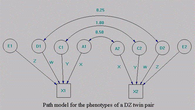
It is a saturated model so the Chi-square fit is zero and none degree of freedom left. Now turn to our neuroticism dataset, we can use MxWin to generate the path diagram (alison.mxd) such as figure 5.5.
The script for ADE model is as follows.
!A D E model fitted
to Alison's Data
G1: model parameters
Data Calc NGroups=4
Begin Matrices;
X Lower 1 1 Free
! genetic structure
Y Lower 1 1 Fixed
! common environmental structure
Z Lower 1 1 Free
! specific environmental structure
W Lower 1 1 Free
! dominance structure
Begin Algebra;
A= X*X' ;
C= Y*Y' ;
E= Z*Z' ;
D= W*W' ;
End Algebra;
End
G2: Monozygotic
twin pairs
Data NInput-vars=2
NObservations=522
LAbels N_T1 N_T2
CMatrix
17.64
8.1421 17.64
Matrices= Group 1
COvariances A+C+D+E
| A+C+D _
A+C+D |
A+C+D+E /
Options RSidual SE
CI=95
END
G3: Dizygotic twin
pairs
Data NInput_vars=2
NObservations=272
LAbels N_T1 N_T2
CMATRIX
18.4599
3.5303 18.4599
MAtrices= GROUP 1
H Full 1 1
Q Full 1 1
Covariances A+C+D+E
| H@A+C+Q@D _
H@A+C+Q@D | A+C+D+E
/
MAtrix H .5
MAtrix Q .25
STart .6 ALL
Options Multiple RSidual
SE CI=95
End
G4: beta-test
DAta calc
MAtrices= Group 1
compute (A|C|D|E) @
(A+C+D+E)~/
Options RS ND=3 SE
CI=95
Options multiple
End
Mx scripts can be split into many groups and allows communication between them, it is thus more flexible than program such as LISREL. The program gives the following estimates.
EXPECTED MATRIX of this
CALCULATION group
1 2
3 4
1
0.279 0.000 0.188
0.533
Example 5.21 Structural equation model analysis assuming complete ascertainment.
!A D E model fitted
to Alison's Data with ascertainment
G1: model parameters
Data Calc NGroups=9
Begin Matrices;
X Lower 1 1 Free
! genetic structure
Y Lower 1 1 Fixed
! common environmental structure
Z Lower 1 1 Free
! specific environmental structure
W Lower 1 1 Free
! dominance structure
M Full 1 2 Fixed
T Full 2 1 Fixed
V Full 2 1 Free
End Matrices
Matrix T 15.5 15.5
Matrix M 10.23 10.23
! Specify M
! 0 0
Begin Algebra;
A= X*X' ;
C= Y*Y' ;
E= Z*Z' ;
D= W*W' ;
V= T-M' ;
End Algebra;
End
G2: Monozygotic
twin pairs
Data NInput-vars=2
NObservations=131
Raw_data file=mz.dat
Labels N_t1 N_t2
Matrices= Group 1
Mean M /
Covariances A+C+D+E
| A+C+D _
A+C+D | A+C+D+E /
Options RSidual
End
G3: dummay group
Data Ninput=2
CTable 2 2
0 0
0 0
! It's full of zeros
so it contributes zero to the function
Matrices = Group 1
Thresholds V /
Covariances A+C+D+E
| A+C+D _
A+C+D | A+C+D+E /
Option RSiduals
End
G4: Calculate ascertainment
correction
Data Ninput=0
Matrices
I Iden 1 1
J Izero 1 2
P Full 2 2 = %P3
T Full 1 1
K Unit 2 1
Compute T*\ln(I-J*P*K)
/
Matrix T 262
! twice the sample size of group 2
Options User-defined
RSiduals Multiple
End
G5: Dizygotic twin
pairs
Data NInput_vars=2
NObservations=75
Raw_data file=dz.dat
Labels N_t1 N_t2
Matrices= Group 1
H Full 1 1
Q Full 1 1
Mean M /
Covariances A+C+D+E
| H@A+C+Q@D _
H@A+C+Q@D | A+C+D+E /
Matrix H .5
Matrix Q .25
Start 3.5 All
Options Multiple RSidual
End
G6: dummy group
Data Ninput=2
CTable 2 2
0 0
0 0
! It's full of zeros
so it contributes zero to the function
Matrices = Group 1
H Full 1 1
Q Full 1 1
Thresholds V /
Covariances A+C+D+E
| H@A+C+Q@D _
H@A+C+Q@D | A+C+D+E /
Matrix H .5
Matrix Q .25
Option RSiduals
End
G7: Calculate ascertainment
correction
Data Ninput=0
Matrices
I Iden 1 1
J Izero 1 2
P Full 2 2 = %P6
T Full 1 1
K Unit 2 1
Compute T*\ln(I-J*P*K)
/
Matrix T 150
! twice the sample size of group 5
Options User-defined
RSiduals Multiple
End
G8: standardization
data calc
matrices= Group 1
compute (A|C|D|E) @
(A+C+D+E)~/
options rs nd=3
options multiple
end
G9: Constraint group
Data Constraint NInput=1
matrices= Group 1
U Full 1 1
Begin Algebra;
S= (X|Y|W|Z);
End Algebra;
Matrix U 18.0
Constraint U - S*S'/
end
The program gives the following estimates for (A, D, E).
EXPECTED MATRIX
of this CALCULATION group
1 2
3 4
1
0.295 0.000 0.166
0.539
The programs allowing for adjustment
of ascertainment are given for ADE,
ACE, AE, DE, CE, and E models, respectively.
Models with means and variances
as free parameters are also given for ADE,
ACE, AE, DE, CE and E only.
Chapter 5 does not provide an example for this. Bonney's regressive models and Haseman-Elston sib pair analysis have been sucessfully implemented in the package SAGE (Statistical Analysis for Genetic Epidemiology). It is composed of series of programs and famous for its capability to include covariates in the analysis. Here we introduce programs FSP, REGC and SIBPAL. FSP is a program for family structure processing. REGC is a program for segregation analysis of continuous trait using regressive models. SIBPAL is a program for Haseman-Elston sib pair analysis.
FSP builds a data structure
for each pedigree, checks pedigree data for correctness of coding,
prepares data for use in SIBPAL and REGC. As of SAGE 2.2, the
typical input and output files for FSP, REGC and SIBPAL are listed
as follows.
Here we set up examples from sage. You can examine these sample files, they are in strict Fortran format. Now you can type name of the program (eg fsp) at DOS prompt, you can issue exit command to return to Windows. We will not go into more details of these programs. Since Fortran refuses to open an existing file for output, you need delete the previous results in order to run the program again. We have a very naive DOS program clean.bat to do this.
Any suggestions and problems
brought to our attention is appreciated.
Pak
Chung Sham and Jing
Hua Zhao 16/2/1998