FM-pipeline

FineMapping analysis using GWAS summary statistics

INTRODUCTION

This is a pipeline for finemapping using GWAS summary statistics, implemented in Bash as a series of steps to furnish an incremental analysis. As depicted in the diagram below

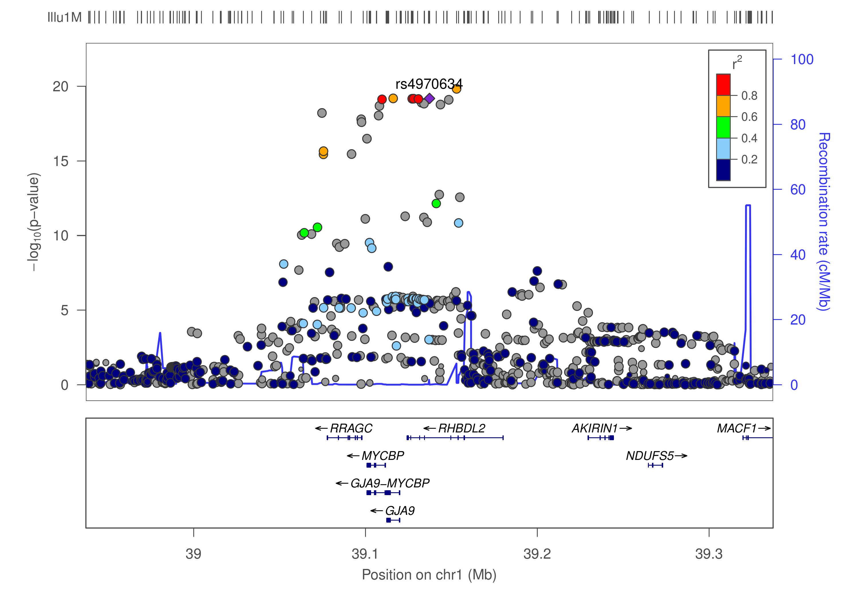
where our lead SNP rs4970634 is in LD with many others, the procedure attempts to identify causal variants from region(s) showing significant SNP-trait association.

The process involves the following steps,

1. Extraction of effect (beta)/z statistics from GWAS summary statistics (.sumstats),
2. Extraction of correlation from the reference panel among overlapped SNPs from 1 and the reference panel containing individual level data.
3. Information from 1 and 2 above is then used as input for finemapping.

The measure of evidence is typically (log10) Bayes factor (BF) and associate SNP probability in the causal set.

It is common to use PLINK and GCTA for identification of independent variants, see ADDTIONAL TOPICS below. Although this pipeline focuses on regional association, these vehicles would offer corroborative information on the regional level, especially when approximately independent LD blocks are used.

Information on whole-genome analysis, which could be used to set up the regions, are described at the wiki page. Clumping using PLINK is also included analogous to those used in depict (e.g. description in PW-pipeline).

INSTALLATION

Software options included in this pipeline are listed in the table below.

Option	Name	Function	Input	Output	Reference
CAVIAR	CAVIAR	finemapping	z, correlation matrix	causal sets and probabilities	Hormozdiari, et al. (2014)
CAVIARBF	CAVIARBF	finemapping	z, correlation matrix	BF and probabilities for all configurations	Chen, et al. (2015)
GCTA	GCTA	joint/conditional analysis	.sumstats, reference data	association results	Yang, et al. (2012)
FM_summary	FM-summary	finemapping	.sumstats	posterior probability & credible set	Huang, et al. (2017)
JAM	JAM	finemapping	beta, individual reference data	Bayes Factor of being causal	Newcombe, et al. (2016)
LocusZoom	LocusZoom	regional plot	.sumstats	.pdf/.png plots	Pruim, et al. (2010)
fgwas	fgwas	functional GWAS	.sumstats	functional significance	Pickrell (2014)
finemap	finemap	finemapping	z, correlation matrix	causal SNPs and configuration	Benner, et al. (2016)

so they range from regional association plots via LocusZoom, joint/conditional analysis via GCTA, functional annotation via fgwas to dedicated finemapping software including CAVIAR, CAVIARBF, an adapted version of FM-summary, R2BGLiMS/JAM and finemap. One can optionally use a subset of these for a particular analysis by specifying relevant flags from the pipeline’s settings.

On many occasions, the pipeline takes advantage of the GNU parallel. Besides (sub)set of software listed in the table above, the pipeline requires qctool 2.0, PLINK 1.9, and the companion program LDstore from finemap’s website need to be installed. To facilitate handling of grapahics, e.g., importing them into Excel, pdftopng from XpdfReader is used. We use Stata and Sun grid engine (sge) for some of the data preparation, which would become handy when available.

The pipeline itself can be installed in the usual way,

git clone https://github.com/jinghuazhao/FM-pipeline

USAGE

An fmp.ini needs to be present at the working directory,

The pipeline is then called with

bash fmp.sh <input>

where <input> is a file containing GWAS summary statistics as described at the SUMSTATS repository, https://github.com/jinghuazhao/SUMSTATS. The input is in line with joint/conditional analysis by GCTA involving chromosomal positions.

The pipeline uses a reference panel in a .gen.gz format, allowing for imputed genotypes and taking into account directions of effect in both the GWAS summary statistics and the reference panel. A .gen.gz file is required for each region, named such that chr{chr}_{start}_{end}.gen.gz, together with an info file and a single .sample file for all regions, see example below.

An auxiliary file called st.bed contains chr, start, end, rsid, pos, r, p corresponding to the lead SNPs specified and r is a sequence number of region while p is a phenotype for GWASs involving multiple phenotyps such as different proteins.

Outputs

The output will involve counterpart(s) from individual software, i.e., .set/.post, .caviarbf, .snp/.config/.cred, .jam/.top/.cs

Software	Output type	Description
CAVIAR	.set/.post	causal set and probabilities in the causal set/posterior probabilities
CAVIARBF	.caviarbf	causal configurations and their BFs
FM-summary	.txt	additional information to the GWAS summary statistics
GCTA	.jma.cojo	joint/conditional analysis results
JAM	.jam/.top/.cs	posterior summary table, top models containing selected SNPs and credible sets
finemap	.snp/.config/.cred	SNPs with largest log10(BF), configurations with their log10(BF) and credible sets

It is helpful to examine directions of effects together with their correlation which is now embedded when finemap is involved.

EXAMPLE

— GWAS summary statistics —

File bmi.tsv.gz is described in the SUMSTATS repository, https://github.com/jinghuazhao/SUMSTATS.

— 1000Genomes panel —

The .gen.gz and .info files for all approximately independent LD blocks are available from 1KG/FUSION, the .sample file is FUSION.sample, all derived from FUSION LD reference panel, with FUSION.sh and FUSION.do.

— The lead SNPs —

From the 97 SNPs described in the SUMSTATS repository, the st.bed is generated as follows,

# 97 SNPs in approximately independent LD blocks
sed -i 's/rs12016871/rs9581854/g' 97.snps
(
  echo -e "chrom\tstart\tend\trsid\tpos\tr"
  grep -w -f 97.snps snp150.txt | \
  sort -k1,1n -k2,2n | \
  awk -vOFS="\t" '{print "chr" $1,$2-1,$2,$3,$2,NR}'
# awk -vflanking=250000 '{l=$2-flanking;u=$2+flanking;if(l<0) l=0;print $1,l,u,$3,$2,NR}'
) | \
bedtools intersect -a 1KG/EUR.bed -b - -loj | \
sed 's/chr//g;s/region//g' | \
(
  echo "chr start end rsid pos r"
  awk '$5!="."{print $1,$2,$3,$8,$9,$4}'
) > st.bed

Note rs12016871 in build 36 became rs9581854 in build 37 and a recent version of bedtools is required to recoggnise standard input. Should we not use approximately independent LD blocks, we would use a flanking region around each SNP as st.bed.

We then proceed with

# modify fmp.ini to use the 1KG panel
gunzip -c bmi.tsv.gz > BMI
fmp.sh BMI

and the results will be in BMI.out.

ADDITIONAL TOPICS

We describe use of PLINK and GCTA to establish regions of interest by first returning to the GIANT BMI example as used above. For PLINK, we do

gunzip -c bmi.tsv.gz | \
sort -k9,9n -k10,10n | \
awk '
{
   OFS="\t"
   if (NR==1) print "SNP","P"
   print $1, $7
}' | \
gzip -f > BMI.P.gz
if [ -f BMI.clumped ]; then rm BMI.clumped; fi
plink --bfile 1KG/FUSION \
      --clump BMI.P.gz \
      --clump-snp-field SNP \
      --clump-field P \
      --clump-kb 500 \
      --clump-p1 5e-8 \
      --clump-p2 0.01 \
      --clump-r2 0.1 \
      --mac 50 \
      --out BMI

where –bfile FUSION contains the LD reference data as from FUSION.sh here. Note that only fields for SNP and p value are required, and for GCTA, we use

gunzip -c bmi.tsv.gz | \
sort -k9,9n -k10,10n | \
awk '
{
   if (NR==1) print "SNP","A1","A2","freq","b","se","p","N"
   print $1, $2, $3, $4, $5, $6, $7, $8
}' > BMI.ma
if [ -f BMI.jma.cojo ]; then rm BMI.jma.cojo BMI.ldr.cojo; fi
gcta64 --bfile 1KG/FUSION \
       --cojo-file BMI.ma \
       --cojo-slct \
       --cojo-p 5e-8 \
       --cojo-collinear 0.01 \
       --cojo-wind 500 \
       --maf 0.0001 \
       --thread-num 3 \
       --out BMI

Since it does not yet accept a compressed file as input.

GCTA is also described on wiki page,

• Whole-genome conditional/joint analysis
• Whole genome analysis using approxmiately independent LD blocks.

The 1000Genomes data above are largely HapMap II SNPs, and a counterpart based on LocusZoom 1.4 and built from lz-1.4.sh increases the number of SNPs from ~1M to ~22M.

RELATED LINK

Credible sets are often described, see https://github.com/statgen/gwas-credible-sets

ACKNOWLEDGEMENTS

The work was motivated by finemapping analysis at the MRC Epidemiology Unit and inputs from authors of GCTA, finemap, JAM, FM-summary as with participants in the Physalia course Practical GWAS Using Linux and R are greatly appreciated. In particular, st.do was adapted from p0.do (which is still used when LD_MAGIC is enabled) originally written by Dr Jian’an Luan and computeCorrelationsImpute2forFINEMAP.r by Ji Chen from the MAGIC consortium who also provides code calculating the credible set based on finemap configurations. Earlier version of the pipeline also used GTOOL.

SOFTWARE AND REFERENCES

CAVIAR (Causal Variants Identification in Associated Regions)

Hormozdiari F, et al. (2014) Identifying causal variants at loci with multiple signals of association. Genetics 44:725–731

CAVIARBF (CAVIAR Bayes Factor)

Chen W, et al. (2015) Fine mapping causal variants with an approximate Bayesian method using marginal test statistics. Genetics 200:719-736.

FM-summary

Huang H, et al (2017) Fine-mapping inflammatory bowel disease loci to single-variant resolution. Nature 547:173–178, doi:10.1038/nature22969

GCTA (Genome-wide Complex Trait Analysis)

Yang J, et al. (2012) Conditional and joint multiple-SNP analysis of GWAS summary statistics identifies additional variants influencing complex traits. Nat Genet 44:369-375

JAM (Joint Analysis of Marginal statistics)

Newcombe PJ, et al. (2016) JAM: A scalable Bayesian framework for joint analysis of marginal SNP effects. Genet Epidemiol 40:188–201

LocusZoom

Pruim RJ, et al. (2010) LocusZoom: Regional visualization of genome-wide association scan results. Bioinformatics 26(18): 2336-2337

fgwas (Functional genomics and genome-wide association studies)

Pickrell JK (2014) Joint analysis of functional genomic data and genome-wide association studies of 18 human traits. Am J Hum Genet 94(4):559-573.

finemap

Benner C, et al. (2016) FINEMAP: Efficient variable selection using summary data from genome-wide association studies. Bioinformatics 32, 1493-1501.

Benner C, et al. (2017) Prospects of fine-mapping trait-associated genomic regions by using summary statistics from genome-wide association studies. Am J Hum Genet 101(4):539-551