This article collects notes on Bioconductor packages, made available here to faciliate their use and extensions.
pkgs <- c("AnnotationDbi", "AnnotationFilter", "ComplexHeatmap", "DESeq2", "EnsDb.Hsapiens.v86",
          "FlowSorted.DLPFC.450k", "GeneNet", "GenomicFeatures", "IlluminaHumanMethylation450kmanifest",
          "OUTRIDER","RColorBrewer", "RMariaDB", "Rgraphviz", "S4Vectors", "SummarizedExperiment",
          "TxDb.Hsapiens.UCSC.hg38.knownGene", "bladderbatch", "clusterProfiler",
          "corpcor", "doParallel", "ensembldb", "fdrtool", "graph", "graphite", "heatmaply",
          "minfi", "org.Hs.eg.db", "plyr", "quantro", "recount3", "sva")
es_pkgs <- c("Biobase", "arrayQualityMetrics", "dplyr", "knitr", "mclust", "pQTLtools", "rgl", "scatterplot3d")
se_pkgs <- c("BiocGenerics", "GenomicRanges", "IRanges", "MsCoreUtils", "SummarizedExperiment", "impute")
sp_pkgs <- c("Biostrings", "CAMERA", "MSnbase", "MSstats", "Spectra", "mzR", "protViz", "rawrr")
pkgs <- c(pkgs, es_pkgs,se_pkgs,sp_pkgs)
for (p in pkgs) if (length(grep(paste("^package:", p, "$", sep=""), search())) == 0) {
    if (!requireNamespace(p)) warning(paste0("This vignette needs package `", p, "'; please install"))
}
invisible(suppressMessages(lapply(pkgs, require, character.only = TRUE)))
1 liftover
See inst/turbomanin the source, https://github.com/jinghuazhao/pQTLtools/tree/master/inst/turboman, or turboman/ directory in the installed package.
2 ExpressionSet
We start with Bioconductor/Biobase’s ExpressionSet example and finish with a real application.
dataDirectory <- system.file("extdata", package="Biobase")
exprsFile <- file.path(dataDirectory, "exprsData.txt")
exprs <- as.matrix(read.table(exprsFile, header=TRUE, sep="\t", row.names=1, as.is=TRUE))
pDataFile <- file.path(dataDirectory, "pData.txt")
pData <- read.table(pDataFile, row.names=1, header=TRUE, sep="\t")
all(rownames(pData)==colnames(exprs))
metadata <- data.frame(labelDescription=c("Patient gender",
                                          "Case/control status",
                                          "Tumor progress on XYZ scale"),
                       row.names=c("gender", "type", "score"))
phenoData <- Biobase::AnnotatedDataFrame(data=pData, varMetadata=metadata)
experimentData <- Biobase::MIAME(name="Pierre Fermat",
                                 lab="Francis Galton Lab",
                                 contact="pfermat@lab.not.exist",
                                 title="Smoking-Cancer Experiment",
                                 abstract="An example ExpressionSet",
                                 url="www.lab.not.exist",
                                 other=list(notes="Created from text files"))
exampleSet <- pQTLtools::make_ExpressionSet(exprs,phenoData,experimentData=experimentData,
                                            annotation="hgu95av2")
data(sample.ExpressionSet, package="Biobase")
identical(exampleSet,sample.ExpressionSet)
2.1 data.frame
The great benefit is to use the object directly as a data.frame.
lm.result <- Biobase::esApply(exampleSet,1,function(x) lm(score~gender+x))
beta.x <- unlist(lapply(lapply(lm.result,coef),"[",3))
beta.x[1]
#> AFFX-MurIL2_at.x
#>    -0.0001907472
lm(score~gender+AFFX.MurIL2_at,data=exampleSet)
#>
#> Call:
#> lm(formula = score ~ gender + AFFX.MurIL2_at, data = exampleSet)
#>
#> Coefficients:
#>    (Intercept)      genderMale  AFFX.MurIL2_at
#>      0.5531725       0.0098932      -0.0001907
2.2 Composite plots
We wish to examine the distribution of each feature via histogram, scatter and boxplot.
One could resort to esApply() for its simplicity as before
invisible(Biobase::esApply(exampleSet[1:2],1,function(x)
                           {par(mfrow=c(3,1));boxplot(x);hist(x);plot(x)}
))
but it is nicer to add feature name in the title.
par(mfrow=c(1,3))
f <- Biobase::featureNames(exampleSet[1:2])
invisible(sapply(f,function(x) {
                     d <- t(Biobase::exprs(exampleSet[x]))
                     fn <- Biobase::featureNames(exampleSet[x])
                     hist(d,main="",xlab=fn); plot(d, ylab=fn); boxplot(d,ylab=fn)
                   }
          )
)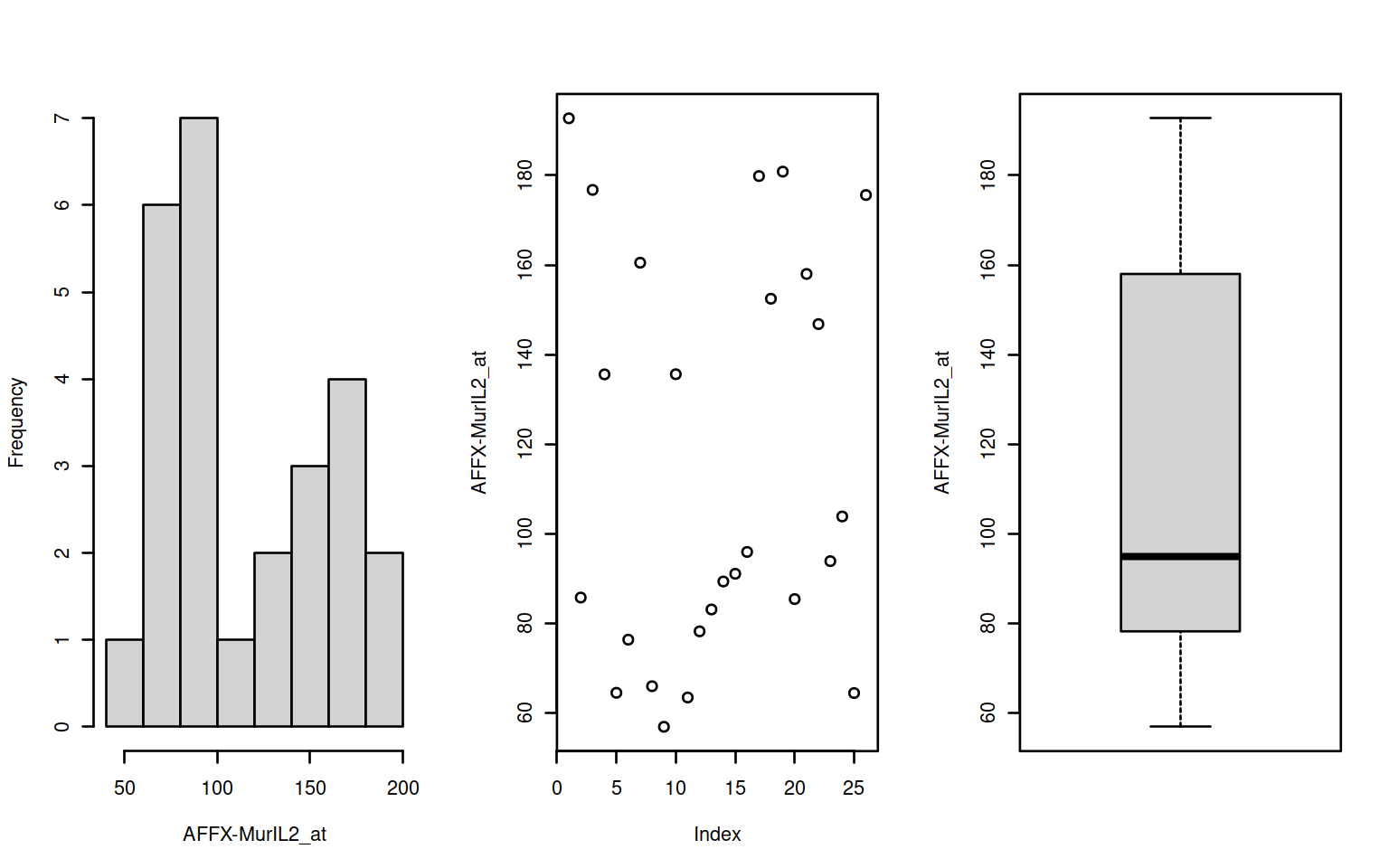
Figure 2.1: Histogram, scatter & boxplots
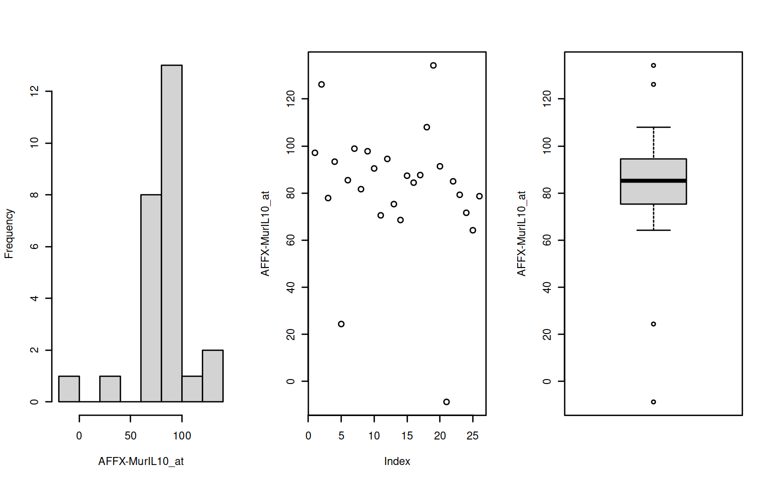
Figure 2.2: Histogram, scatter & boxplots
where the expression set is indexed using feature name(s).
2.4 Clustering
We employ model-based clustering absed on principal compoents to see potential groupings in the data,
  pca <- prcomp(na.omit(t(Biobase::exprs(exampleSet))), rank=10, scale=TRUE)
  pc1pc2pc3 <- with(pca,x)[,1:3]
  mc <- mclust::Mclust(pc1pc2pc3,G=3)
  with(mc, {
      cols <- c("blue","red", "purple")
      s3d <- scatterplot3d::scatterplot3d(with(pca,x[,c(2,1,3)]),
                                          color=cols[classification],
                                          pch=16,
                                          type="h",
                                          main="Plot of the PC1, PC2 and PC3")
      s3d.coords <- s3d$xyz.convert(with(pca,x[,c(2,1,3)]))
      text(s3d.coords$x,
           s3d.coords$y,
           cex = 1.2,
           col = cols[classification],
           labels = row.names(pc1pc2pc3),
           pos = 4)
      legend("right", legend=levels(as.factor(classification)), col=cols[classification], pch=16)
      rgl::open3d(width = 500, height = 500)
      rgl::plot3d(with(pca,x[,c(2,1,3)]),cex=1.2,col=cols[classification],size=5)
      rgl::text3d(with(pca,x[,c(2,1,3)]),cex=1.2,col=cols[classification],texts=row.names(pc1pc2pc3))
      widget <- rgl::rglwidget()
      htmlwidgets::saveWidget(widget, "mcpca3d.html")
  })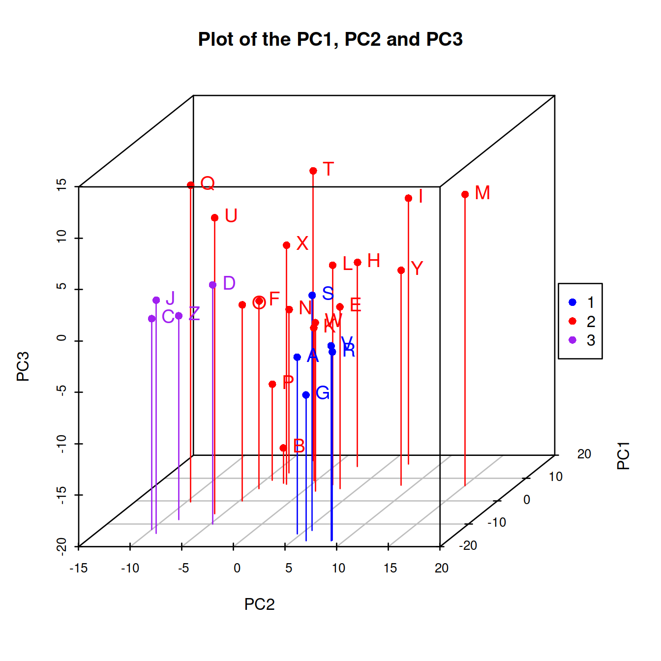
Figure 2.3: Three-group Clustering
#> Warning in par3d(userMatrix = structure(c(1, 0, 0, 0, 0, 0.342020143325668, :
#> parameter "width" cannot be set
#> Warning in par3d(userMatrix = structure(c(1, 0, 0, 0, 0, 0.342020143325668, :
#> parameter "height" cannot be set
An interactive version is also available,
2.5 Data transformation
Suppose we wish use log2 for those greater than zero but set those negative values to be missing.
2.6 Limit of detection (LOD)
We generate a lod.max ~ U[0,1] variable to experiment
data(sample.ExpressionSet, package = "Biobase")
exampleSet <- sample.ExpressionSet
set.seed(1)
probs <- runif(nrow(exampleSet))
Biobase::fData(exampleSet)$lod.max <- vapply(seq_len(nrow(exampleSet)), function(i)
           quantile(Biobase::exprs(exampleSet)[i, ], probs = probs[i], na.rm = TRUE),
           numeric(1))
lod <- get.prop.below.LLOD(exampleSet)
fd <- Biobase::fData(lod)
fd <- fd[order(fd$pc.belowLOD.new, decreasing = TRUE), ]
knitr::kable(head(fd))| lod.max | pc.belowLOD.new | |
|---|---|---|
| AFFX-BioC-3_st | 130.21243 | 96.15385 |
| 31319_at | 166.52127 | 96.15385 |
| 31343_at | 23.26079 | 96.15385 |
| 31350_at | 276.87575 | 96.15385 |
| 31360_at | 68.95543 | 96.15385 |
| 31378_at | 143.30260 | 96.15385 |
plot(fd$pc.belowLOD.new, main = "Random quantile cut off", ylab = "% below LOD")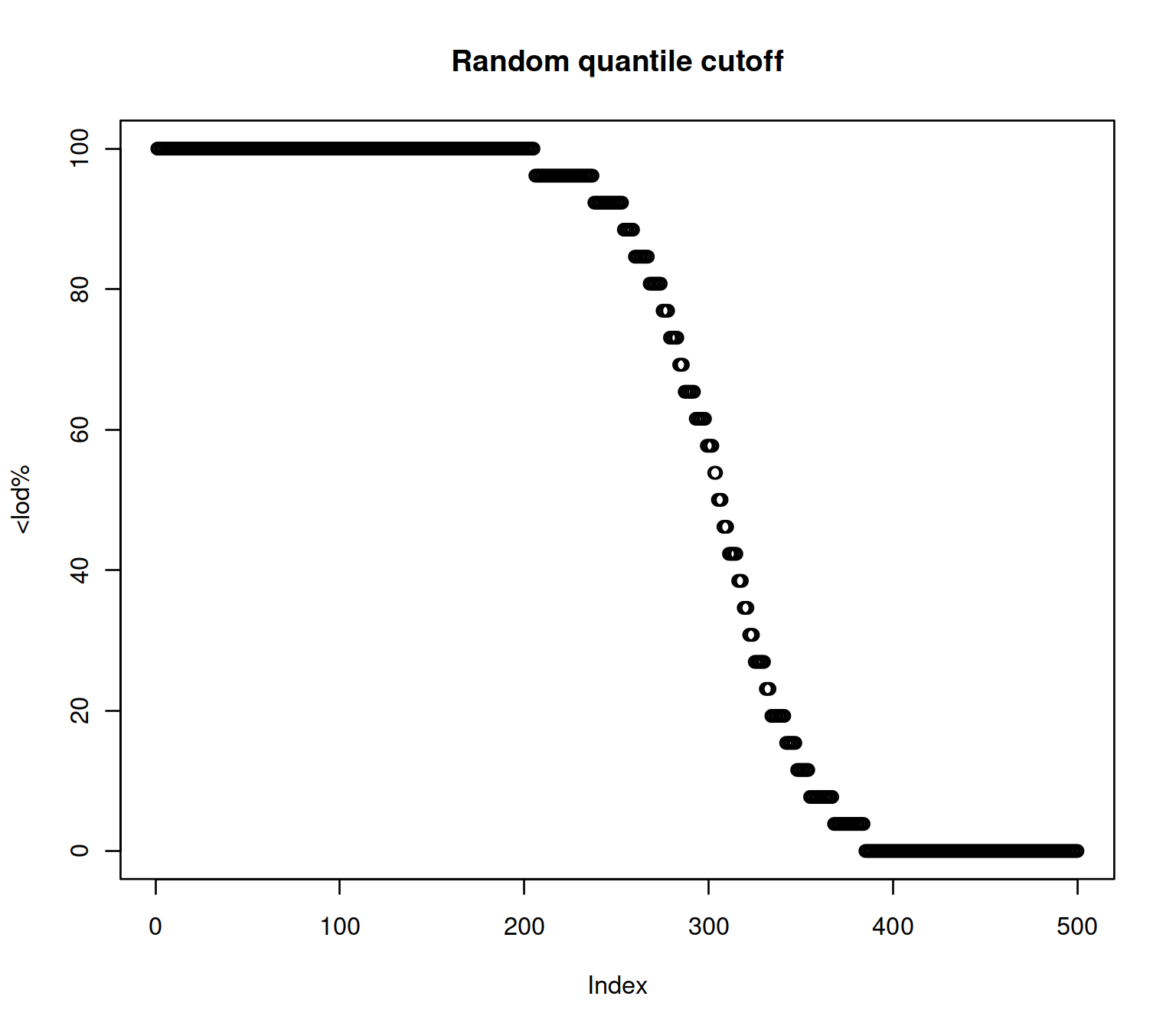
Figure 2.4: LOD based on a random cutoff
The quantity has been shown to have a big impact on protein abundance and therefore pQTL detection as is shown with a real example.
rm(list=ls())
dir <- "~/rds/post_qc_data/interval/phenotype/olink_proteomics/post-qc/"
eset <- readRDS(paste0(dir,"eset.inf1.flag.out.outlier.in.rds"))
x <- pQTLtools::get.prop.below.LLOD(eset)
annot <- Biobase::fData(x)
annot$MissDataProp <- as.numeric(gsub("\\%$", "", annot$MissDataProp))
plot(annot$MissDataProp, annot$pc.belowLOD.new, xlab="% <LLOD in Original",
     ylab="% <LLOD in post QC dataset", pch=19)
INF <- Sys.getenv("INF")
np <- read.table(paste(INF, "work", "INF1.merge.nosig", sep="/"), header=FALSE,
                 col.names = c("prot", "uniprot"))
kable(np, caption="Proteins with no pQTL")
annot$pQTL <- rep(NA, nrow(annot))
no.pQTL.ind <- which(annot$uniprot.id %in% np$uniprot)
annot$pQTL[no.pQTL.ind] <- "red"
annot$pQTL[-no.pQTL.ind] <- "blue"
annot <- annot[order(annot$pc.belowLOD.new, decreasing = TRUE),]
annot <- annot[-grep("^BDNF$", annot$ID),]
saveRDS(annot,file=file.path("~","pQTLtools","tests","annot.RDS"))
annot <- readRDS(file.path(find.package("pQTLtools"),"tests","annot.RDS")) %>%
         dplyr::left_join(pQTLdata::inf1[c("prot","target.short","alt_name")],by=c("ID"="prot")) %>%
         dplyr::mutate(prot=if_else(is.na(alt_name),target.short,alt_name),order=1:n()) %>%
         dplyr::arrange(desc(order))
xtick <- seq(1, nrow(annot))
attach(annot)
par(mar=c(10,5,1,1))
plot(100-pc.belowLOD.new,cex=2,pch=19,col=pQTL,xaxt="n",xlab="",ylab="",cex.axis=0.8)
text(66,16,"IL-17C",offset=0,pos=2,cex=1.5,font=2,srt=0)
arrows(67,16,71,16,lwd=2)
axis(1, at=xtick, labels=prot, lwd.tick=0.5, lwd=0, las=2, hadj=1, cex.axis=0.8)
mtext("% samples above LLOD",side=2,line=2.5,cex=1.2)
mtext("Ordered protein",side=1,line=6.5,cex=1.2,font=1)
legend(x=1,y=25,c("without pQTL","with pQTL"),box.lwd=0,cex=2,col=c("red","blue"),pch=19)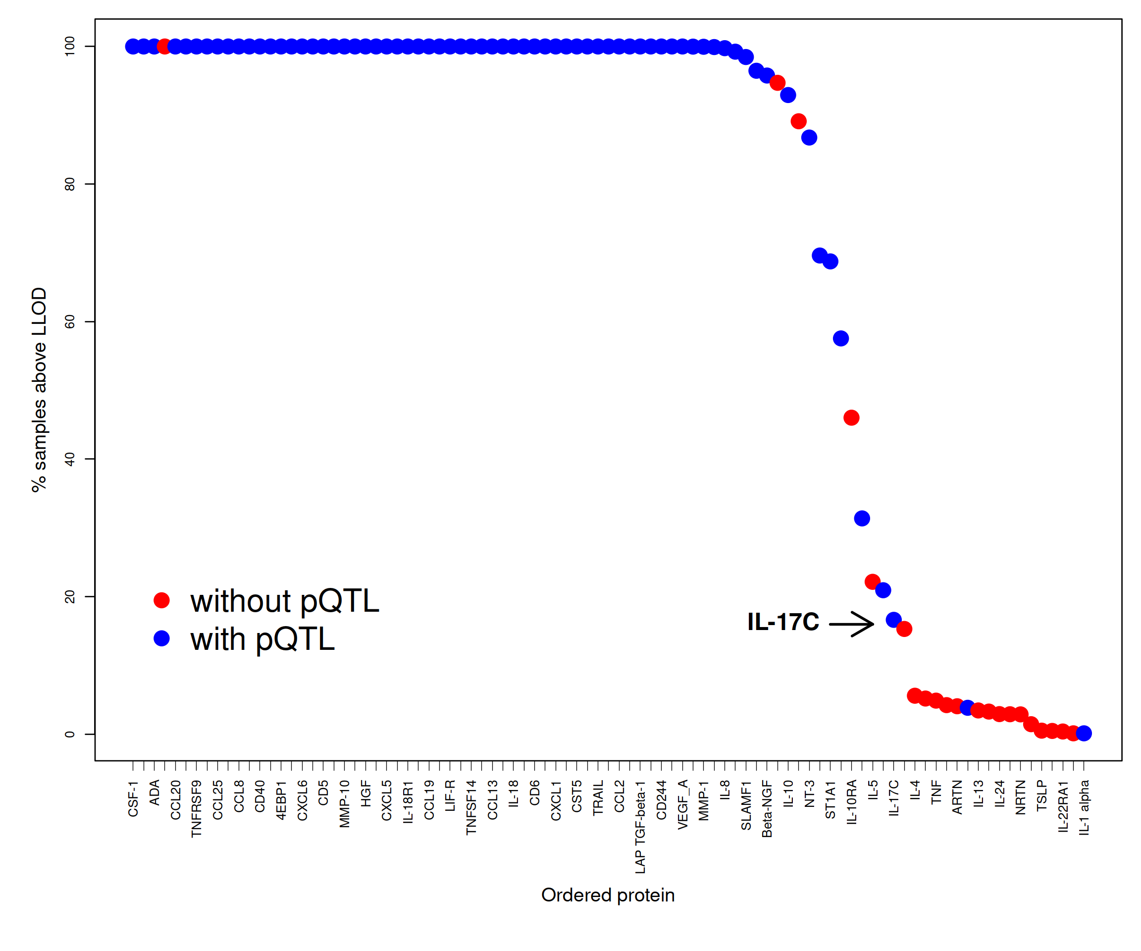
Figure 2.5: LOD in SCALLOP-INF/INTERVAL
| ID | dichot | olink.id | uniprot.id | lod.max | MissDataProp | pc.belowLOD.new | pQTL | target.short | alt_name | prot | order |
|---|---|---|---|---|---|---|---|---|---|---|---|
| CSF.1 | FALSE | 196_CSF-1 | P09603 | 1.02 | 0.02 | 0.0000000 | blue | CSF-1 | NA | CSF-1 | 91 |
| TNFB | FALSE | 195_TNFB | P01374 | 1.10 | 0.04 | 0.0000000 | blue | TNFB | NA | TNFB | 90 |
| ADA | FALSE | 194_ADA | P00813 | 1.80 | 0.04 | 0.0000000 | blue | ADA | NA | ADA | 89 |
| STAMPB | FALSE | 192_STAMPB | O95630 | 1.40 | 0.06 | 0.0000000 | red | STAMPB | NA | STAMPB | 88 |
| CCL20 | FALSE | 190_CCL20 | P78556 | 1.42 | 0.02 | 0.0000000 | blue | CCL20 | NA | CCL20 | 87 |
| TWEAK | FALSE | 189_TWEAK | O43508 | 1.78 | 0.02 | 0.0000000 | blue | TWEAK | NA | TWEAK | 86 |
| TNFRSF9 | FALSE | 187_TNFRSF9 | Q07011 | 1.86 | 0.02 | 0.0000000 | blue | TNFRSF9 | NA | TNFRSF9 | 85 |
| CX3CL1 | FALSE | 186_CX3CL1 | P78423 | 1.76 | 0.02 | 0.0000000 | blue | CX3CL1 | NA | CX3CL1 | 84 |
| CCL25 | FALSE | 185_CCL25 | O15444 | 1.32 | 0.02 | 0.0000000 | blue | CCL25 | NA | CCL25 | 83 |
| CASP.8 | FALSE | 184_CASP-8 | Q14790 | 1.38 | 0.04 | 0.0000000 | blue | CASP-8 | NA | CASP-8 | 82 |
| MCP.2 | FALSE | 183_MCP-2 | P80075 | 2.10 | 0.02 | 0.0000000 | blue | MCP-2 | CCL8 | CCL8 | 81 |
| FGF.19 | FALSE | 179_FGF-19 | O95750 | 1.25 | 0.02 | 0.0000000 | blue | FGF-19 | NA | FGF-19 | 80 |
| CD40 | FALSE | 176_CD40 | P25942 | 1.91 | 0.04 | 0.0000000 | blue | CD40 | NA | CD40 | 79 |
| DNER | FALSE | 174_DNER | Q8NFT8 | 1.63 | 0.02 | 0.0000000 | blue | DNER | NA | DNER | 78 |
| 4E.BP1 | FALSE | 170_4E-BP1 | Q13541 | 1.04 | 0.10 | 0.0000000 | blue | 4EBP1 | NA | 4EBP1 | 77 |
| CXCL10 | FALSE | 169_CXCL10 | P02778 | 2.03 | 0.02 | 0.0000000 | blue | CXCL10 | NA | CXCL10 | 76 |
| CXCL6 | FALSE | 168_CXCL6 | P80162 | 1.80 | 0.02 | 0.0000000 | blue | CXCL6 | CXCL6 | CXCL6 | 75 |
| Flt3L | FALSE | 167_Flt3L | P49771 | 2.12 | 0.02 | 0.0000000 | blue | FIt3L | NA | FIt3L | 74 |
| CD5 | FALSE | 165_CD5 | P06127 | 1.42 | 0.02 | 0.0000000 | blue | CD5 | NA | CD5 | 73 |
| CCL23 | FALSE | 164_CCL23 | P55773 | 2.10 | 0.02 | 0.0000000 | blue | CCL23 | NA | CCL23 | 72 |
| MMP.10 | FALSE | 161_MMP-10 | P09238 | 1.56 | 0.02 | 0.0000000 | blue | MMP-10 | NA | MMP-10 | 71 |
| IL.12B | FALSE | 157_IL-12B | P29460 | 0.85 | 0.02 | 0.0000000 | blue | IL-12B | NA | IL-12B | 70 |
| HGF | FALSE | 156_HGF | P14210 | 1.77 | 0.02 | 0.0000000 | blue | HGF | NA | HGF | 69 |
| TRANCE | FALSE | 155_TRANCE | O14788 | 1.51 | 0.04 | 0.0000000 | blue | TRANCE | NA | TRANCE | 68 |
| CXCL5 | FALSE | 154_CXCL5 | P42830 | 1.92 | 0.02 | 0.0000000 | blue | CXCL5 | NA | CXCL5 | 67 |
| PD.L1 | FALSE | 152_PD-L1 | Q9NZQ7 | 2.14 | 0.04 | 0.0000000 | blue | PD-L1 | NA | PD-L1 | 66 |
| IL.18R1 | FALSE | 151_IL-18R1 | Q13478 | 1.21 | 0.02 | 0.0000000 | blue | IL-18R1 | NA | IL-18R1 | 65 |
| IL.10RB | FALSE | 149_IL-10RB | Q08334 | 1.72 | 0.02 | 0.0000000 | blue | IL10RB | NA | IL10RB | 64 |
| CCL19 | FALSE | 145_CCL19 | Q99731 | 2.13 | 0.02 | 0.0000000 | blue | CCL19 | NA | CCL19 | 63 |
| FGF.21 | FALSE | 144_FGF-21 | Q9NSA1 | 1.14 | 0.02 | 0.0000000 | blue | FGF-21 | NA | FGF-21 | 62 |
| LIF.R | FALSE | 143_LIF-R | P42702 | 2.08 | 0.04 | 0.0000000 | blue | LIF-R | NA | LIF-R | 61 |
| FGF.23 | FALSE | 139_FGF-23 | Q9GZV9 | 0.66 | 0.04 | 0.0000000 | blue | FGF-23 | NA | FGF-23 | 60 |
| TNFSF14 | FALSE | 138_TNFSF14 | O43557 | 1.81 | 0.02 | 0.0000000 | blue | TNFSF14 | NA | TNFSF14 | 59 |
| CCL11 | FALSE | 137_CCL11 | P51671 | 2.09 | 0.02 | 0.0000000 | blue | CCL11 | CCL11 | CCL11 | 58 |
| MCP.4 | FALSE | 136_MCP-4 | Q99616 | 0.56 | 0.04 | 0.0000000 | blue | MCP-4 | CCL13 | CCL13 | 57 |
| TGF.alpha | FALSE | 135_TGF-alpha | P01135 | 0.07 | 0.02 | 0.0000000 | blue | TGF-alpha | NA | TGF-alpha | 56 |
| IL.18 | FALSE | 133_IL-18 | Q14116 | 2.79 | 0.02 | 0.0000000 | blue | IL-18 | NA | IL-18 | 55 |
| SCF | FALSE | 132_SCF | P21583 | 2.30 | 0.02 | 0.0000000 | blue | SCF | NA | SCF | 54 |
| CD6 | FALSE | 131_CD6 | Q8WWJ7 | 1.78 | 0.04 | 0.0000000 | blue | CD6 | NA | CD6 | 53 |
| CCL4 | FALSE | 130_CCL4 | P13236 | 2.15 | 0.02 | 0.0000000 | blue | CCL4 | NA | CCL4 | 52 |
| CXCL1 | FALSE | 128_CXCL1 | P09341 | 3.45 | 0.02 | 0.0000000 | blue | CXCL1 | NA | CXCL1 | 51 |
| OSM | FALSE | 126_OSM | P13725 | 1.32 | 0.06 | 0.0000000 | blue | OSM | NA | OSM | 50 |
| CST5 | FALSE | 123_CST5 | P28325 | 4.34 | 0.04 | 0.0000000 | blue | CST5 | NA | CST5 | 49 |
| CXCL9 | FALSE | 122_CXCL9 | Q07325 | 1.04 | 0.02 | 0.0000000 | blue | CXCL9 | NA | CXCL9 | 48 |
| TRAIL | FALSE | 120_TRAIL | P50591 | 1.22 | 0.02 | 0.0000000 | blue | TRAIL | NA | TRAIL | 47 |
| CXCL11 | FALSE | 117_CXCL11 | O14625 | 1.40 | 0.02 | 0.0000000 | blue | CXCL11 | NA | CXCL11 | 46 |
| MCP.1 | FALSE | 115_MCP-1 | P13500 | 1.90 | 0.02 | 0.0000000 | blue | MCP-1 | CCL2 | CCL2 | 45 |
| uPA | FALSE | 112_uPA | P00749 | 1.75 | 0.02 | 0.0000000 | blue | uPA | NA | uPA | 44 |
| LAP.TGF.beta.1 | FALSE | 111_LAP TGF-beta-1 | P01137 | 0.86 | 0.02 | 0.0000000 | blue | LAP TGF-beta-1 | NA | LAP TGF-beta-1 | 43 |
| OPG | FALSE | 110_OPG | O00300 | 1.81 | 0.02 | 0.0000000 | blue | OPG | NA | OPG | 42 |
| CD244 | FALSE | 108_CD244 | Q9BZW8 | 1.09 | 0.02 | 0.0000000 | blue | CD244 | NA | CD244 | 41 |
| CDCP1 | FALSE | 107_CDCP1 | Q9H5V8 | 0.21 | 0.04 | 0.0000000 | blue | CDCP1 | NA | CDCP1 | 40 |
| VEGF.A | FALSE | 102_VEGF-A | P15692 | 3.15 | 0.02 | 0.0000000 | blue | VEGF_A | NA | VEGF_A | 39 |
| MIP.1.alpha | FALSE | 166_MIP-1 alpha | P10147 | 1.92 | 0.06 | 0.0203998 | blue | MIP-1 alpha | NA | MIP-1 alpha | 38 |
| MMP.1 | FALSE | 142_MMP-1 | P03956 | 1.89 | 0.06 | 0.0407997 | blue | MMP-1 | NA | MMP-1 | 37 |
| SIRT2 | FALSE | 172_SIRT2 | Q8IXJ6 | 1.52 | 1.00 | 0.0815993 | blue | SIRT2 | NA | SIRT2 | 36 |
| IL.8 | FALSE | 101_IL-8 | P10145 | 3.17 | 0.25 | 0.2447980 | blue | IL-8 | NA | IL-8 | 35 |
| IL.7 | FALSE | 109_IL-7 | P13232 | 1.39 | 1.43 | 0.7547940 | blue | IL-7 | NA | IL-7 | 34 |
| SLAMF1 | FALSE | 134_SLAMF1 | Q13291 | 1.55 | 2.13 | 1.5299878 | blue | SLAMF1 | NA | SLAMF1 | 33 |
| EN.RAGE | FALSE | 175_EN-RAGE | P80511 | 1.57 | 3.28 | 3.5291718 | blue | EN-RAGE | NA | EN-RAGE | 32 |
| Beta.NGF | FALSE | 153_Beta-NGF | P01138 | 1.23 | 3.96 | 4.2227662 | blue | Beta-NGF | NA | Beta-NGF | 31 |
| CCL28 | FALSE | 173_CCL28 | Q9NRJ3 | 0.92 | 5.49 | 5.2835577 | red | CCL28 | NA | CCL28 | 30 |
| IL.10 | FALSE | 162_IL-10 | P22301 | 1.50 | 7.71 | 7.0583435 | blue | IL-10 | NA | IL-10 | 29 |
| AXIN1 | FALSE | 118_AXIN1 | O15169 | 1.30 | 13.04 | 10.8731130 | red | AXIN1 | NA | AXIN1 | 28 |
| NT.3 | FALSE | 188_NT-3 | P20783 | 0.85 | 12.77 | 13.2394941 | blue | NT-3 | NA | NT-3 | 27 |
| FGF.5 | FALSE | 141_FGF-5 | Q8NF90 | 1.00 | 31.71 | 30.3957568 | blue | FGF-5 | NA | FGF-5 | 26 |
| ST1A1 | FALSE | 191_ST1A1 | P50225 | 1.34 | 32.68 | 31.2525500 | blue | ST1A1 | NA | ST1A1 | 25 |
| GDNF | FALSE | 106_GDNF | P39905 | 1.13 | 43.26 | 42.4520604 | blue | hGDNF | NA | hGDNF | 24 |
| IL.10RA | FALSE | 140_IL-10RA | Q13651 | 1.14 | 53.30 | 53.9779682 | red | IL-10RA | NA | IL-10RA | 23 |
| IL.6 | FALSE | 113_IL-6 | P05231 | 1.97 | 69.06 | 68.6250510 | blue | IL-6 | NA | IL-6 | 22 |
| IL.5 | FALSE | 193_IL-5 | P05113 | 1.55 | 78.21 | 77.8457772 | red | IL-5 | NA | IL-5 | 21 |
| MCP.3 | FALSE | 105_MCP-3 | P80098 | 1.31 | 79.30 | 79.0697674 | blue | MCP-3 | CCL7 | CCL7 | 20 |
| IL.17C | FALSE | 114_IL-17C | Q9P0M4 | 1.28 | 83.07 | 83.3741330 | blue | IL-17C | NA | IL-17C | 19 |
| IL.17A | FALSE | 116_IL-17A | Q16552 | 0.97 | 84.73 | 84.7001224 | red | IL-17A | NA | IL-17A | 18 |
| IL.4 | FALSE | 180_IL-4 | P05112 | 1.11 | 93.91 | 94.4104447 | red | IL-4 | NA | IL-4 | 17 |
| LIF | FALSE | 181_LIF | P15018 | 1.45 | 94.90 | 94.8184415 | red | LIF | NA | LIF | 16 |
| TNF | FALSE | 163_TNF | P01375 | 1.19 | 95.22 | 95.1244390 | red | TNF | NA | TNF | 15 |
| IL.20RA | FALSE | 121_IL-20RA | Q9UHF4 | 0.79 | 95.16 | 95.7772338 | red | IL-20RA | NA | IL-20RA | 14 |
| ARTN | FALSE | 160_ARTN | Q5T4W7 | 0.73 | 95.84 | 95.9404325 | red | ARTN | NA | ARTN | 13 |
| IL.15RA | FALSE | 148_IL-15RA | Q13261 | 1.18 | 96.10 | 96.1648307 | blue | IL-15RA | NA | IL-15RA | 12 |
| IL.13 | FALSE | 159_IL-13 | P35225 | 1.71 | 96.51 | 96.5524276 | red | IL-13 | NA | IL-13 | 11 |
| IL.20 | FALSE | 171_IL-20 | Q9NYY1 | 1.30 | 96.72 | 96.7156263 | red | IL-20 | NA | IL-20 | 10 |
| IL.24 | FALSE | 158_IL-24 | Q13007 | 1.95 | 97.13 | 97.0828233 | red | IL-24 | NA | IL-24 | 9 |
| IL.2RB | FALSE | 124_IL-2RB | P14784 | 1.47 | 97.11 | 97.1032232 | red | IL-2RB | NA | IL-2RB | 8 |
| NRTN | FALSE | 182_NRTN | Q99748 | 1.39 | 97.11 | 97.1236230 | red | NRTN | NA | NRTN | 7 |
| IL.33 | FALSE | 177_IL-33 | O95760 | 1.17 | 98.54 | 98.5516116 | red | IL-33 | NA | IL-33 | 6 |
| TSLP | FALSE | 129_TSLP | Q969D9 | 1.80 | 99.49 | 99.4900041 | red | TSLP | NA | TSLP | 5 |
| IFN.gamma | FALSE | 178_IFN-gamma | P01579 | 1.40 | 99.53 | 99.5308038 | red | IFN-gamma | NA | IFN-gamma | 4 |
| IL.22.RA1 | FALSE | 150_IL-22 RA1 | Q8N6P7 | 1.79 | 99.61 | 99.6124031 | red | IL-22RA1 | NA | IL-22RA1 | 3 |
| IL.2 | FALSE | 127_IL-2 | P60568 | 0.93 | 99.86 | 99.8776010 | red | IL-2 | NA | IL-2 | 2 |
| IL.1.alpha | FALSE | 125_IL-1 alpha | P01583 | 4.76 | 99.88 | 99.8776010 | blue | IL-1 alpha | NA | IL-1 alpha | 1 |
2.7 maEndtoEnd
Web: https://bioconductor.org/packages/release/workflows/html/maEndToEnd.html.
Examples can be found on PCA, heatmap, normalisation, linear models, and enrichment analysis from this Bioconductor package.
3 SummarizedExperiment
This is a more modern construct. Based on the documentation example, ranged summarized experiment (rse) and imputation are shown below.
set.seed(123)
nrows <- 20
ncols <- 4
counts <- matrix(runif(nrows * ncols, 1, 1e4), nrows)
missing_indices <- sample(length(counts), size = 5, replace = FALSE)
counts[missing_indices] <- NA
rowRanges <- GenomicRanges::GRanges(rep(c("chr1", "chr2"), c(1, 3) * nrows / 4),
                            IRanges::IRanges(floor(runif(nrows, 1e5, 1e6)), width=ncols),
                            strand=sample(c("+", "-"), nrows, TRUE),
                            feature_id=sprintf("ID%03d", 1:nrows))
colData <- S4Vectors::DataFrame(Treatment=rep(c("ChIP", "Input"), ncols/2),
                                row.names=LETTERS[1:ncols])
rse <- SummarizedExperiment::SummarizedExperiment(assays=S4Vectors::SimpleList(counts=counts),
                                                  rowRanges=rowRanges, colData=colData)
SummarizedExperiment::assay(rse)
#>               A         B         C           D
#>  [1,] 2876.4876 8895.5036 1428.8574 6651.486831
#>  [2,] 7883.2630 6928.3413 4146.0488  949.311769
#>  [3,] 4090.3602 6405.4276 4137.8295 3840.312408
#>  [4,] 8830.2910 9942.7035 3689.0857 2744.562062
#>  [5,] 9404.7324 6557.4023 1525.2950 8146.585749
#>  [6,]        NA 7085.5962 1388.9218 4485.714898
#>  [7,] 5281.5268 5441.1162 2331.1080 8100.833466
#>  [8,] 8924.2980 5941.8261 4660.1585 8124.082706
#>  [9,] 5514.7987 2892.3082 2660.4604 7943.628869
#> [10,] 4566.6907 1471.9894        NA 4398.877044
#> [11,] 9568.3766        NA  459.2658 7544.997111
#> [12,] 4533.8882 9023.0882 4422.5585          NA
#> [13,] 6776.0288 6907.3621 7989.4495 7102.113831
#> [14,] 5726.7614 7954.8787 1219.8707    7.247108
#> [15,] 1030.1439  247.1122 5609.9189 4753.690424
#> [16,] 8998.3499 4778.4819 2066.1074 2201.968733
#> [17,] 2461.6313 7584.8369 1276.1890 3798.785561
#> [18,]  421.5533 2164.8630 7533.3253 6128.097262
#> [19,] 3279.8793        NA 8950.5585 3518.627295
#> [20,] 9545.0820 2317.0262 3745.2533 1112.243108
imputed <- MsCoreUtils::impute_knn(as.matrix(SummarizedExperiment::assay(rse)),2)
imputed_counts <- MsCoreUtils::impute_RF(as.matrix(SummarizedExperiment::assay(rse)),2)
imputed-imputed_counts
#>              A          B        C        D
#>  [1,]    0.000     0.0000    0.000    0.000
#>  [2,]    0.000     0.0000    0.000    0.000
#>  [3,]    0.000     0.0000    0.000    0.000
#>  [4,]    0.000     0.0000    0.000    0.000
#>  [5,]    0.000     0.0000    0.000    0.000
#>  [6,] 1661.249     0.0000    0.000    0.000
#>  [7,]    0.000     0.0000    0.000    0.000
#>  [8,]    0.000     0.0000    0.000    0.000
#>  [9,]    0.000     0.0000    0.000    0.000
#> [10,]    0.000     0.0000 1632.214    0.000
#> [11,]    0.000 -1253.3641    0.000    0.000
#> [12,]    0.000     0.0000    0.000 3109.097
#> [13,]    0.000     0.0000    0.000    0.000
#> [14,]    0.000     0.0000    0.000    0.000
#> [15,]    0.000     0.0000    0.000    0.000
#> [16,]    0.000     0.0000    0.000    0.000
#> [17,]    0.000     0.0000    0.000    0.000
#> [18,]    0.000     0.0000    0.000    0.000
#> [19,]    0.000   745.3773    0.000    0.000
#> [20,]    0.000     0.0000    0.000    0.000
SummarizedExperiment::assays(rse) <- S4Vectors::SimpleList(counts=imputed_counts)
SummarizedExperiment::assay(rse)
#>               A         B         C           D
#>  [1,] 2876.4876 8895.5036 1428.8574 6651.486831
#>  [2,] 7883.2630 6928.3413 4146.0488  949.311769
#>  [3,] 4090.3602 6405.4276 4137.8295 3840.312408
#>  [4,] 8830.2910 9942.7035 3689.0857 2744.562062
#>  [5,] 9404.7324 6557.4023 1525.2950 8146.585749
#>  [6,] 5337.3847 7085.5962 1388.9218 4485.714898
#>  [7,] 5281.5268 5441.1162 2331.1080 8100.833466
#>  [8,] 8924.2980 5941.8261 4660.1585 8124.082706
#>  [9,] 5514.7987 2892.3082 2660.4604 7943.628869
#> [10,] 4566.6907 1471.9894 4972.0817 4398.877044
#> [11,] 9568.3766 6089.8420  459.2658 7544.997111
#> [12,] 4533.8882 9023.0882 4422.5585 3970.354132
#> [13,] 6776.0288 6907.3621 7989.4495 7102.113831
#> [14,] 5726.7614 7954.8787 1219.8707    7.247108
#> [15,] 1030.1439  247.1122 5609.9189 4753.690424
#> [16,] 8998.3499 4778.4819 2066.1074 2201.968733
#> [17,] 2461.6313 7584.8369 1276.1890 3798.785561
#> [18,]  421.5533 2164.8630 7533.3253 6128.097262
#> [19,] 3279.8793 5119.1973 8950.5585 3518.627295
#> [20,] 9545.0820 2317.0262 3745.2533 1112.243108
SummarizedExperiment::assays(rse) <- S4Vectors::endoapply(SummarizedExperiment::assays(rse), asinh)
SummarizedExperiment::assay(rse)
#>              A        B        C        D
#>  [1,] 8.657472 9.786448 7.957778 9.495743
#>  [2,] 9.665644 9.536523 9.023058 7.548885
#>  [3,] 9.009536 9.458048 9.021074 8.946456
#>  [4,] 9.779090 9.897741 8.906281 8.610524
#>  [5,] 9.842115 9.481497 8.023090 9.698501
#>  [6,] 9.275638 9.558966 7.929430 9.101800
#>  [7,] 9.265118 9.294887 8.447246 9.692869
#>  [8,] 9.789680 9.382919 9.139952 9.695735
#>  [9,] 9.308338 8.662957 8.579402 9.673273
#> [10,] 9.119691 7.987517 9.204741 9.082252
#> [11,] 9.859366 9.407525 6.822778 9.621787
#> [12,] 9.112482 9.800689 9.087621 8.979758
#> [13,] 9.514294 9.533490 9.679024 9.561295
#> [14,] 9.346053 9.674688 7.799647 2.678476
#> [15,] 7.630601 6.202994 9.325439 9.159824
#> [16,] 9.797944 9.165025 8.326569 8.390254
#> [17,] 8.501727 9.627054 7.844781 8.935584
#> [18,] 6.737095 8.373260 9.620239 9.413787
#> [19,] 8.788709 9.233900 9.792618 8.858973
#> [20,] 9.856929 8.441187 8.921392 7.707281

SummarizedExperiment::rowRanges(rse)
#> GRanges object with 20 ranges and 1 metadata column:
#>        seqnames        ranges strand |  feature_id
#>           <Rle>     <IRanges>  <Rle> | <character>
#>    [1]     chr1 409164-409167      - |       ID001
#>    [2]     chr1 691082-691085      + |       ID002
#>    [3]     chr1 388335-388338      + |       ID003
#>    [4]     chr1 268922-268925      - |       ID004
#>    [5]     chr1 804064-804067      - |       ID005
#>    ...      ...           ...    ... .         ...
#>   [16]     chr2 647861-647864      + |       ID016
#>   [17]     chr2 469620-469623      + |       ID017
#>   [18]     chr2 232385-232388      + |       ID018
#>   [19]     chr2 941769-941772      - |       ID019
#>   [20]     chr2 371106-371109      + |       ID020
#>   -------
#>   seqinfo: 2 sequences from an unspecified genome; no seqlengths
SummarizedExperiment::rowData(rse)
#> DataFrame with 20 rows and 1 column
#>      feature_id
#>     <character>
#> 1         ID001
#> 2         ID002
#> 3         ID003
#> 4         ID004
#> 5         ID005
#> ...         ...
#> 16        ID016
#> 17        ID017
#> 18        ID018
#> 19        ID019
#> 20        ID020
SummarizedExperiment::colData(rse)
#> DataFrame with 4 rows and 1 column
#>     Treatment
#>   <character>
#> A        ChIP
#> B       Input
#> C        ChIP
#> D       Input
4 Normalisation
4.1 ComBat
This is the documentation example, based on Bioconductor 3.14.
data(bladderdata, package="bladderbatch")
edat <- bladderEset[1:50]

pheno <- Biobase::pData(edat)
batch <- pheno$batch
table(batch)
#> batch
#>  1  2  3  4  5
#> 11 18  4  5 19
quantro::matboxplot(edat,batch,cex.axis=0.6,notch=TRUE,pch=19,ylab="Expression")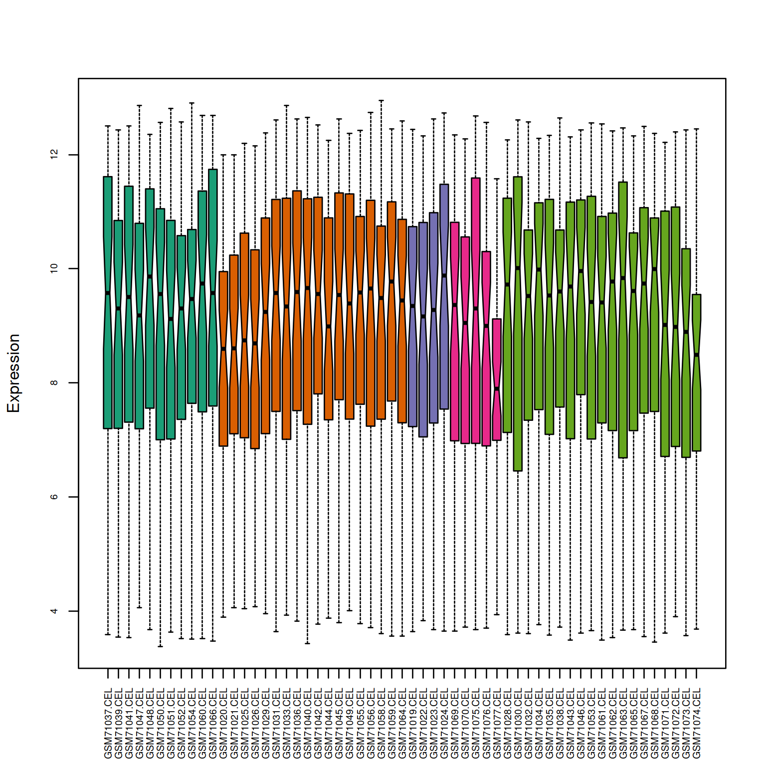
Figure 4.1: ComBat example
quantro::matdensity(edat,batch,xlab=" ",ylab="density")
legend("topleft",legend=1:5,col=1:5,lty=1)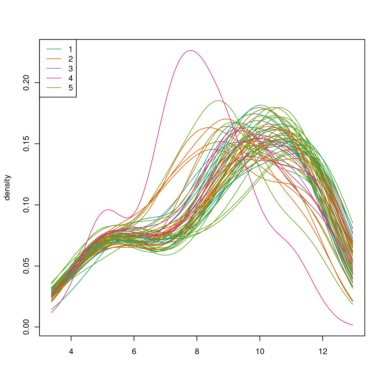
Figure 4.2: ComBat example
# 1. parametric adjustment
combat_edata1 <- sva::ComBat(dat=edat, batch=batch, par.prior=TRUE, prior.plots=TRUE)
#> Found5batches
#> Adjusting for0covariate(s) or covariate level(s)
#> Standardizing Data across genes
#> Fitting L/S model and finding priors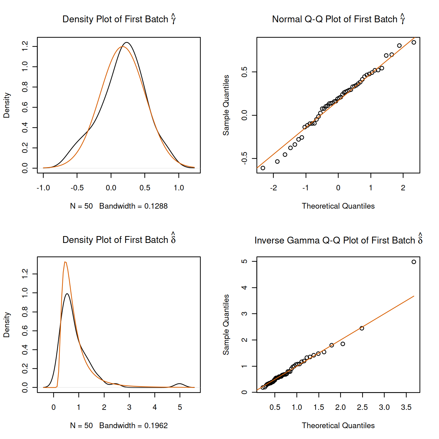
Figure 4.3: ComBat example
#> Finding parametric adjustments
#> Adjusting the Data

# 2. non-parametric adjustment, mean-only version
combat_edata2 <- sva::ComBat(dat=edat, batch=batch, par.prior=FALSE, mean.only=TRUE)
#> Using the 'mean only' version of ComBat
#> Found5batches
#> Adjusting for0covariate(s) or covariate level(s)
#> Standardizing Data across genes
#> Fitting L/S model and finding priors
#> Finding nonparametric adjustments
#> Adjusting the Data

# 3. reference-batch version, with covariates
mod <- model.matrix(~as.factor(cancer), data=pheno)
combat_edata3 <- sva::ComBat(dat=edat, batch=batch, mod=mod, par.prior=TRUE, ref.batch=3, prior.plots=TRUE)
#> Using batch =3as a reference batch (this batch won't change)
#> Found5batches
#> Adjusting for2covariate(s) or covariate level(s)
#> Standardizing Data across genes
#> Fitting L/S model and finding priors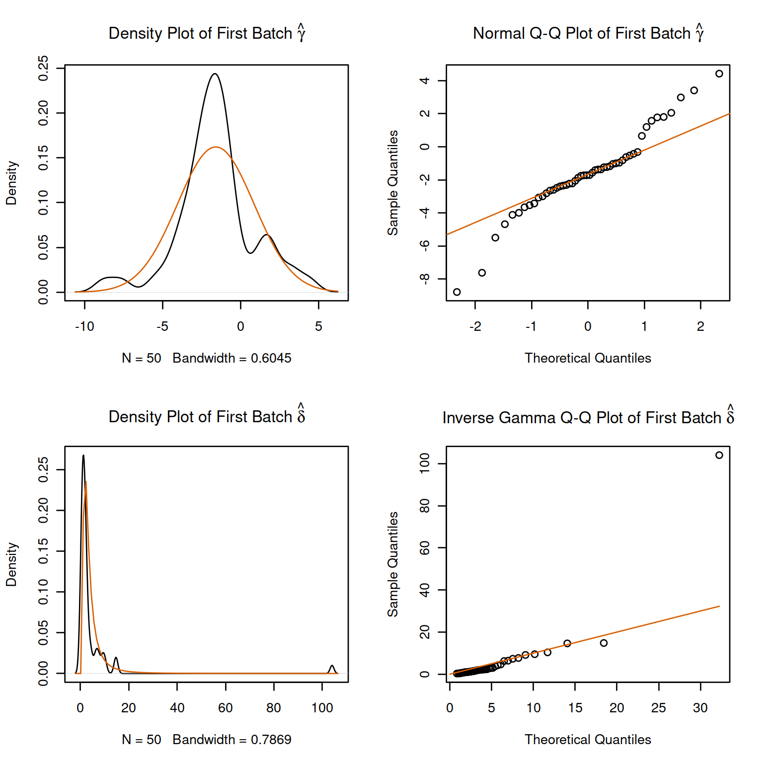
Figure 4.4: ComBat example
#> Finding parametric adjustments
#> Adjusting the Data
4.2 quantro
This is also adapted from the package vignette but with FlowSorted.DLPFC.450k in place of FlowSorted.
data(FlowSorted.DLPFC.450k,package="FlowSorted.DLPFC.450k")
p <- getBeta(FlowSorted.DLPFC.450k,offset=100)
pd <- Biobase::pData(FlowSorted.DLPFC.450k)
quantro::matboxplot(p, groupFactor = pd$CellType, xaxt = "n", main = "Beta Values", pch=19)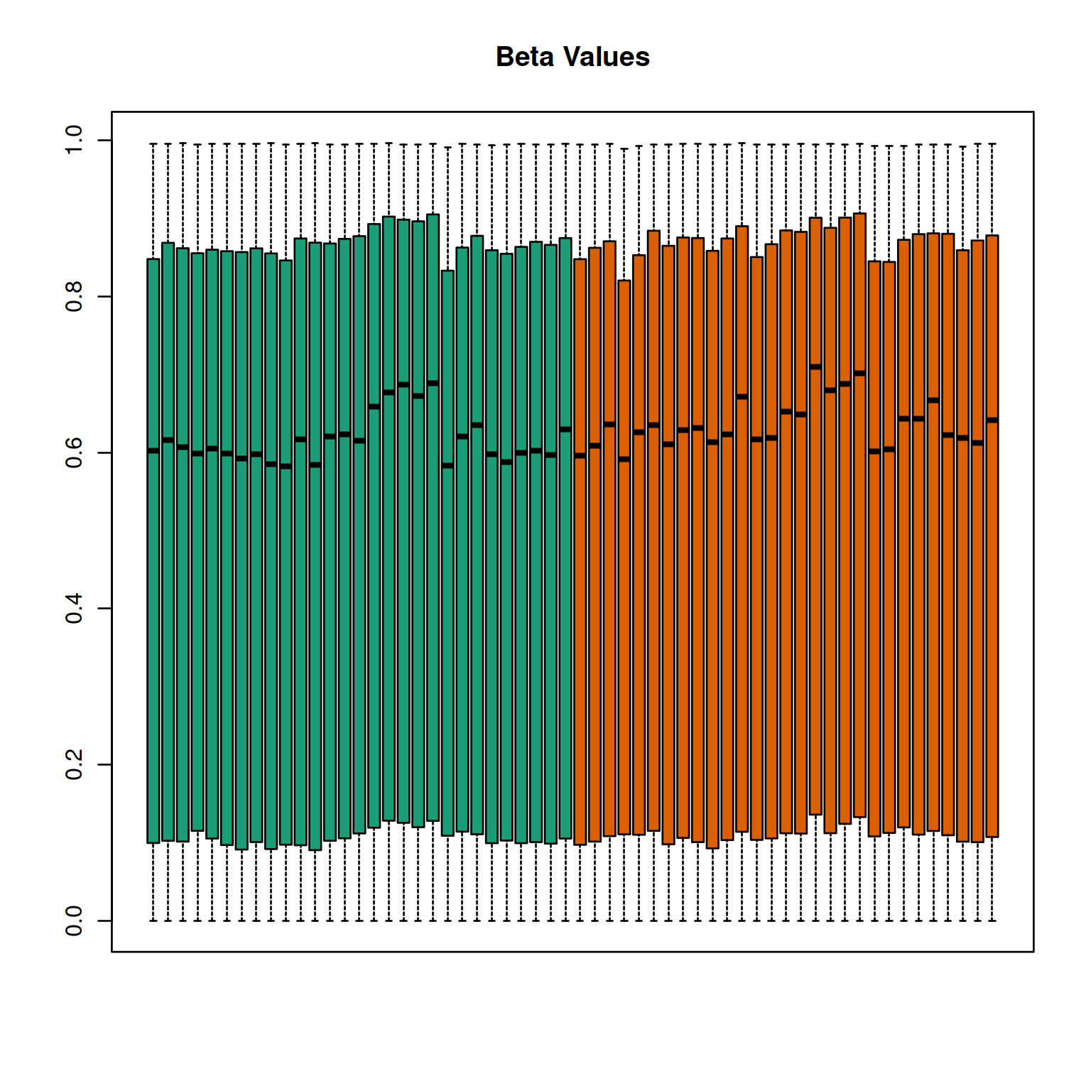
Figure 4.5: quantro example
quantro::matdensity(p, groupFactor = pd$CellType, xlab = " ", ylab = "density",
                    main = "Beta Values", brewer.n = 8, brewer.name = "Dark2")
legend('top', c("NeuN_neg", "NeuN_pos"), col = c(1, 2), lty = 1, lwd = 3)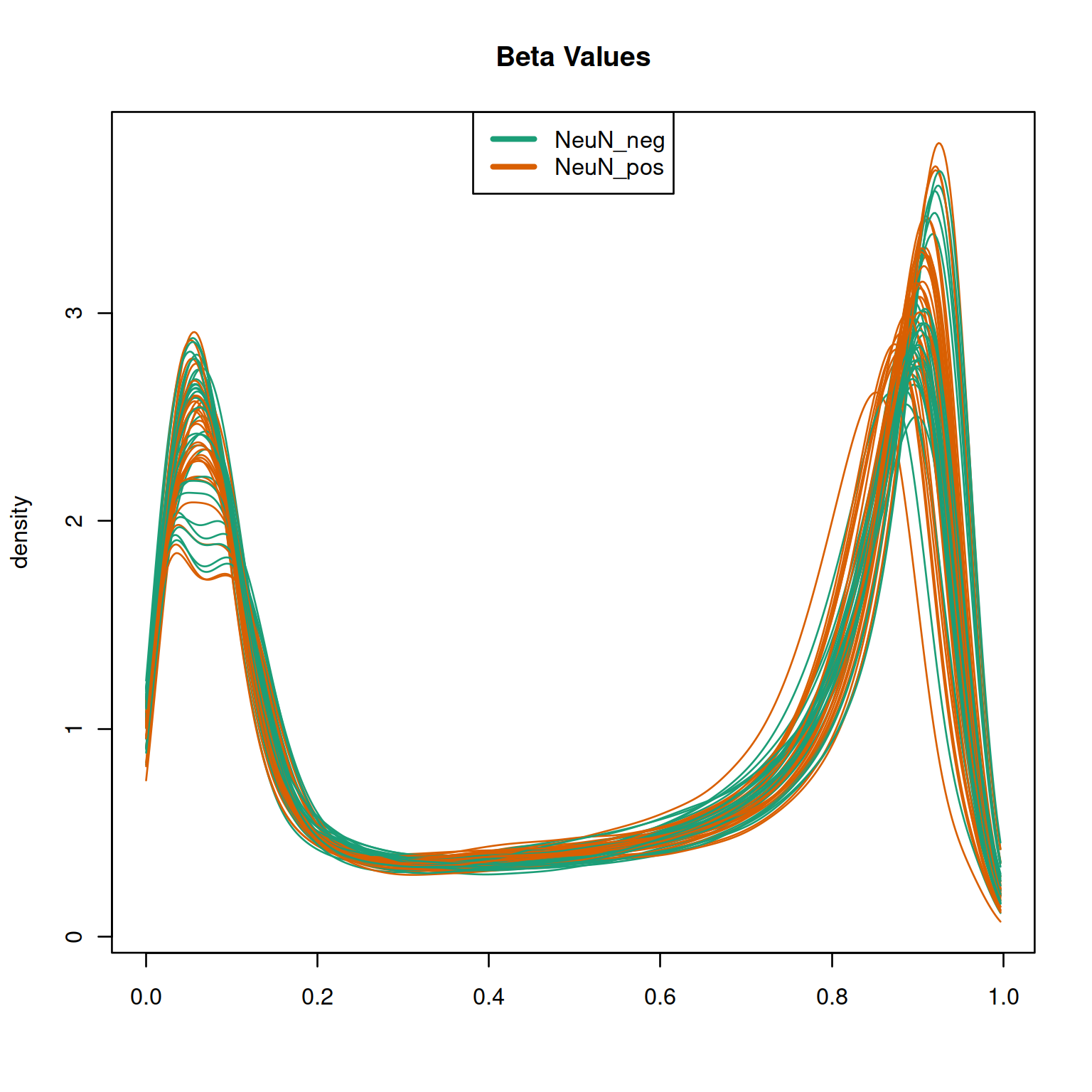
Figure 4.6: quantro example
qtest <- quantro::quantro(object = p, groupFactor = pd$CellType)
#> [quantro] Average medians of the distributions are
#>                         not equal across groups.
#> [quantro] Calculating the quantro test statistic.
#> [quantro] No permutation testing performed.
#>                          Use B > 0 for permutation testing.
if (FALSE)
{
  doParallel::registerDoParallel(cores=10)
  qtestPerm <- quantro::quantro(p, groupFactor = pd$CellType, B = 1000)
  quantro::quantroPlot(qtestPerm)
}
5 Outlier detection in RNA-Seq
The following is adapted from package OUTRIDER, noting its plotQQ() has issues
ctsFile <- system.file('extdata', 'KremerNBaderSmall.tsv', package='OUTRIDER')
ctsTable <- read.table(ctsFile, check.names=FALSE)
ods <- OUTRIDER::OutriderDataSet(countData=ctsTable)
ods <- OUTRIDER::filterExpression(ods, minCounts=TRUE, filterGenes=TRUE)
ods <- OUTRIDER::OUTRIDER(ods)
res <- OUTRIDER::results(ods)
knitr::kable(res,caption="A check list of outliers")
if ("geneID" %in% colnames(res) & FALSE)
  OUTRIDER::plotQQ(ods, res$geneID, global=TRUE)
6 Differential expression
ex <- DESeq2::makeExampleDESeqDataSet(m=4)
dds <- DESeq2::DESeq(ex)
#> estimating size factors
#> estimating dispersions
#> gene-wise dispersion estimates
#> mean-dispersion relationship
#> final dispersion estimates
#> fitting model and testing
res <- DESeq2::results(dds, contrast=c("condition","B","A"))
rld <- DESeq2::rlogTransformation(ex, blind=TRUE)
dat <- DESeq2::plotPCA(rld, intgroup=c("condition"),returnData=TRUE)
#> using ntop=500 top features by variance
percentVar <- round(100 * attr(dat,"percentVar"))
ggplot2::ggplot(dat, ggplot2::aes(PC1, PC2, color=condition, shape=condition)) +
ggplot2::geom_point(size=3) +
ggplot2::xlab(paste0("PC1:",percentVar[1],"% variance")) +
ggplot2::ylab(paste0("PC2:",percentVar[2],"% variance"))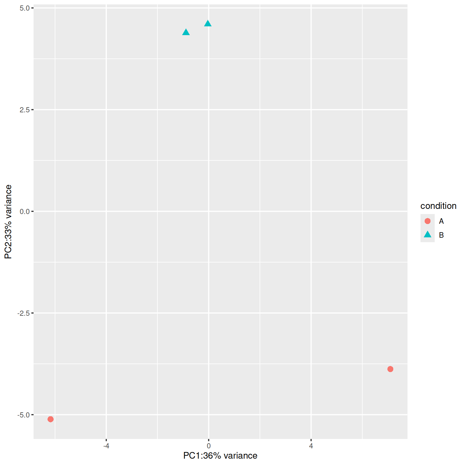
Figure 6.1: DESeq2 example
ex$condition <- relevel(ex$condition, ref="B")
dds2 <- DESeq2::DESeq(dds)
#> using pre-existing size factors
#> estimating dispersions
#> found already estimated dispersions, replacing these
#> gene-wise dispersion estimates
#> mean-dispersion relationship
#> final dispersion estimates
#> fitting model and testing
res <- DESeq2::results(dds2)
knitr::kable(head(as.data.frame(res)))| baseMean | log2FoldChange | lfcSE | stat | pvalue | padj | |
|---|---|---|---|---|---|---|
| gene1 | 32.066278 | 0.6915335 | 0.8953643 | 0.7723488 | 0.4399079 | 0.9961926 |
| gene2 | 4.412314 | -1.0016303 | 2.0623610 | -0.4856717 | 0.6272000 | 0.9961926 |
| gene3 | 30.498821 | -0.9328430 | 0.8577129 | -1.0875936 | 0.2767745 | 0.9961926 |
| gene4 | 36.510796 | -0.9515118 | 0.8692174 | -1.0946764 | 0.2736584 | 0.9961926 |
| gene5 | 4.622864 | 3.0727212 | 2.1197063 | 1.4495976 | 0.1471708 | 0.9961926 |
| gene6 | 39.111363 | -1.1866091 | 0.7171454 | -1.6546282 | 0.0979999 | 0.9961926 |
See the package in action from a snakemake workflow1.
7 Gene co-expression and network analysis
A simple network is furnished with the GeneNet documentation example,
## A random network with 40 nodes
# it contains 780=40*39/2 edges of which 5 percent (=39) are non-zero
true.pcor <- GeneNet::ggm.simulate.pcor(40)

# A data set with 40 observations
m.sim <- GeneNet::ggm.simulate.data(40, true.pcor)

# A simple estimate of partial correlations
estimated.pcor <- corpcor::cor2pcor( cor(m.sim) )

# A comparison of estimated and true values
sum((true.pcor-estimated.pcor)^2)
#> [1] 259.8131

# A slightly better estimate ...
estimated.pcor.2 <- GeneNet::ggm.estimate.pcor(m.sim)
#> Estimating optimal shrinkage intensity lambda (correlation matrix): 0.1511
sum((true.pcor-estimated.pcor.2)^2)
#> [1] 12.37069

## ecoli data
data(ecoli, package="GeneNet")

# partial correlation matrix
inferred.pcor <- GeneNet::ggm.estimate.pcor(ecoli)
#> Estimating optimal shrinkage intensity lambda (correlation matrix): 0.1804

# p-values, q-values and posterior probabilities for each potential edge
test.results <- GeneNet::network.test.edges(inferred.pcor)
#> Estimate (local) false discovery rates (partial correlations):
#> Step 1... determine cutoff point
#> Step 2... estimate parameters of null distribution and eta0
#> Step 3... compute p-values and estimate empirical PDF/CDF
#> Step 4... compute q-values and local fdr
#> Step 5... prepare for plotting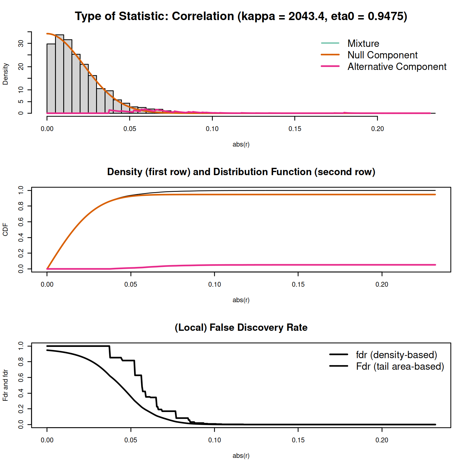
Figure 7.1: GeneNet example
# best 20 edges (strongest correlation)
test.results[1:20,]
#>           pcor node1 node2         pval         qval      prob
#> 1   0.23185664    51    53 2.220446e-16 3.612205e-13 1.0000000
#> 2   0.22405545    52    53 2.220446e-16 3.612205e-13 1.0000000
#> 3   0.21507824    51    52 2.220446e-16 3.612205e-13 1.0000000
#> 4   0.17328863     7    93 3.108624e-15 3.792816e-12 0.9999945
#> 5  -0.13418892    29    86 1.120812e-09 1.093997e-06 0.9999516
#> 6   0.12594697    21    72 1.103836e-08 8.978563e-06 0.9998400
#> 7   0.11956105    28    86 5.890924e-08 3.853590e-05 0.9998400
#> 8  -0.11723897    26    80 1.060526e-07 5.816172e-05 0.9998400
#> 9  -0.11711625    72    89 1.093655e-07 5.930499e-05 0.9972804
#> 10  0.10658013    20    21 1.366610e-06 5.925275e-04 0.9972804
#> 11  0.10589778    21    73 1.596859e-06 6.678429e-04 0.9972804
#> 12  0.10478689    20    91 2.053403e-06 8.024425e-04 0.9972804
#> 13  0.10420836     7    52 2.338382e-06 8.778605e-04 0.9944557
#> 14  0.10236077    87    95 3.525186e-06 1.224964e-03 0.9944557
#> 15  0.10113550    27    95 4.610444e-06 1.500047e-03 0.9920084
#> 16  0.09928954    21    51 6.868357e-06 2.046549e-03 0.9920084
#> 17  0.09791914    21    88 9.192373e-06 2.520616e-03 0.9920084
#> 18  0.09719685    18    95 1.070232e-05 2.790102e-03 0.9920084
#> 19  0.09621791    28    90 1.313007e-05 3.171817e-03 0.9920084
#> 20  0.09619099    12    80 1.320374e-05 3.182526e-03 0.9920084

# network containing edges with prob > 0.9 (i.e. local fdr < 0.1)
net <- GeneNet::extract.network(test.results, cutoff.ggm=0.9)
#>
#> Significant edges:  65
#>     Corresponding to  1.26 %  of possible edges
net
#>           pcor node1 node2         pval         qval      prob
#> 1   0.23185664    51    53 2.220446e-16 3.612205e-13 1.0000000
#> 2   0.22405545    52    53 2.220446e-16 3.612205e-13 1.0000000
#> 3   0.21507824    51    52 2.220446e-16 3.612205e-13 1.0000000
#> 4   0.17328863     7    93 3.108624e-15 3.792816e-12 0.9999945
#> 5  -0.13418892    29    86 1.120812e-09 1.093997e-06 0.9999516
#> 6   0.12594697    21    72 1.103836e-08 8.978563e-06 0.9998400
#> 7   0.11956105    28    86 5.890924e-08 3.853590e-05 0.9998400
#> 8  -0.11723897    26    80 1.060526e-07 5.816172e-05 0.9998400
#> 9  -0.11711625    72    89 1.093655e-07 5.930499e-05 0.9972804
#> 10  0.10658013    20    21 1.366610e-06 5.925275e-04 0.9972804
#> 11  0.10589778    21    73 1.596859e-06 6.678429e-04 0.9972804
#> 12  0.10478689    20    91 2.053403e-06 8.024425e-04 0.9972804
#> 13  0.10420836     7    52 2.338382e-06 8.778605e-04 0.9944557
#> 14  0.10236077    87    95 3.525186e-06 1.224964e-03 0.9944557
#> 15  0.10113550    27    95 4.610444e-06 1.500047e-03 0.9920084
#> 16  0.09928954    21    51 6.868357e-06 2.046549e-03 0.9920084
#> 17  0.09791914    21    88 9.192373e-06 2.520616e-03 0.9920084
#> 18  0.09719685    18    95 1.070232e-05 2.790102e-03 0.9920084
#> 19  0.09621791    28    90 1.313007e-05 3.171817e-03 0.9920084
#> 20  0.09619099    12    80 1.320374e-05 3.182526e-03 0.9920084
#> 21  0.09576091    89    95 1.443542e-05 3.354777e-03 0.9891317
#> 22  0.09473210     7    51 1.784126e-05 3.864825e-03 0.9891317
#> 23 -0.09386896    53    58 2.127622e-05 4.313590e-03 0.9891317
#> 24 -0.09366615    29    83 2.217013e-05 4.421099e-03 0.9891317
#> 25 -0.09341148    21    89 2.334321e-05 4.556947e-03 0.9810727
#> 26 -0.09156391    49    93 3.380043e-05 5.955972e-03 0.9810727
#> 27 -0.09150710    80    90 3.418363e-05 6.002083e-03 0.9810727
#> 28  0.09101505     7    53 3.767966e-05 6.408102e-03 0.9810727
#> 29  0.09050688    21    84 4.164471e-05 6.838782e-03 0.9810727
#> 30  0.08965490    72    73 4.919365e-05 7.581866e-03 0.9810727
#> 31 -0.08934025    29    99 5.229604e-05 7.861416e-03 0.9810727
#> 32 -0.08906819     9    95 5.512708e-05 8.104759e-03 0.9810727
#> 33  0.08888345     2    49 5.713144e-05 8.270673e-03 0.9810727
#> 34  0.08850681    86    90 6.143363e-05 8.610161e-03 0.9810727
#> 35  0.08805868    17    53 6.695170e-05 9.015175e-03 0.9810727
#> 36  0.08790809    28    48 6.890884e-05 9.151291e-03 0.9810727
#> 37  0.08783471    33    58 6.988211e-05 9.217597e-03 0.9682377
#> 38 -0.08705796     7    49 8.101244e-05 1.021362e-02 0.9682377
#> 39  0.08645033    20    46 9.086547e-05 1.102466e-02 0.9682377
#> 40  0.08609950    48    86 9.705862e-05 1.150392e-02 0.9682377
#> 41  0.08598769    21    52 9.911458e-05 1.165816e-02 0.9682377
#> 42  0.08555275    32    95 1.075099e-04 1.226435e-02 0.9682377
#> 43  0.08548231    17    51 1.089311e-04 1.236337e-02 0.9424721
#> 44  0.08470370    80    83 1.258659e-04 1.382356e-02 0.9424721
#> 45  0.08442510    80    82 1.325062e-04 1.437068e-02 0.9174573
#> 46  0.08271606    80    93 1.810275e-04 1.845632e-02 0.9174573
#> 47  0.08235175    46    91 1.933329e-04 1.941579e-02 0.9174573
#> 48  0.08217787    25    95 1.994788e-04 1.988432e-02 0.9174573
#> 49 -0.08170331    29    87 2.171999e-04 2.119715e-02 0.9174573
#> 50  0.08123632    19    29 2.360716e-04 2.253606e-02 0.9174573
#> 51  0.08101702    51    84 2.454547e-04 2.318024e-02 0.9174573
#> 52  0.08030748    16    93 2.782643e-04 2.532796e-02 0.9174573
#> 53  0.08006503    28    52 2.903870e-04 2.608271e-02 0.9174573
#> 54 -0.07941656    41    80 3.252833e-04 2.814824e-02 0.9174573
#> 55  0.07941410    54    89 3.254229e-04 2.815620e-02 0.9174573
#> 56 -0.07934653    28    80 3.292784e-04 2.837511e-02 0.9174573
#> 57  0.07916783    29    92 3.396802e-04 2.895702e-02 0.9174573
#> 58 -0.07866905    17    86 3.703635e-04 3.060293e-02 0.9174573
#> 59  0.07827749    16    29 3.962446e-04 3.191462e-02 0.9174573
#> 60 -0.07808262    73    89 4.097452e-04 3.257290e-02 0.9174573
#> 61  0.07766261    52    67 4.403165e-04 3.400207e-02 0.9174573
#> 62  0.07762917    25    87 4.428396e-04 3.411637e-02 0.9174573
#> 63 -0.07739378     9    93 4.609872e-04 3.492295e-02 0.9174573
#> 64  0.07738885    31    80 4.613747e-04 3.493988e-02 0.9174573
#> 65 -0.07718681    80    94 4.775136e-04 3.563444e-02 0.9174573

# significant based on FDR cutoff Q=0.05?
num.significant.1 <- sum(test.results$qval <= 0.05)
test.results[1:num.significant.1,]
#>           pcor node1 node2         pval         qval      prob
#> 1   0.23185664    51    53 2.220446e-16 3.612205e-13 1.0000000
#> 2   0.22405545    52    53 2.220446e-16 3.612205e-13 1.0000000
#> 3   0.21507824    51    52 2.220446e-16 3.612205e-13 1.0000000
#> 4   0.17328863     7    93 3.108624e-15 3.792816e-12 0.9999945
#> 5  -0.13418892    29    86 1.120812e-09 1.093997e-06 0.9999516
#> 6   0.12594697    21    72 1.103836e-08 8.978563e-06 0.9998400
#> 7   0.11956105    28    86 5.890924e-08 3.853590e-05 0.9998400
#> 8  -0.11723897    26    80 1.060526e-07 5.816172e-05 0.9998400
#> 9  -0.11711625    72    89 1.093655e-07 5.930499e-05 0.9972804
#> 10  0.10658013    20    21 1.366610e-06 5.925275e-04 0.9972804
#> 11  0.10589778    21    73 1.596859e-06 6.678429e-04 0.9972804
#> 12  0.10478689    20    91 2.053403e-06 8.024425e-04 0.9972804
#> 13  0.10420836     7    52 2.338382e-06 8.778605e-04 0.9944557
#> 14  0.10236077    87    95 3.525186e-06 1.224964e-03 0.9944557
#> 15  0.10113550    27    95 4.610444e-06 1.500047e-03 0.9920084
#> 16  0.09928954    21    51 6.868357e-06 2.046549e-03 0.9920084
#> 17  0.09791914    21    88 9.192373e-06 2.520616e-03 0.9920084
#> 18  0.09719685    18    95 1.070232e-05 2.790102e-03 0.9920084
#> 19  0.09621791    28    90 1.313007e-05 3.171817e-03 0.9920084
#> 20  0.09619099    12    80 1.320374e-05 3.182526e-03 0.9920084
#> 21  0.09576091    89    95 1.443542e-05 3.354777e-03 0.9891317
#> 22  0.09473210     7    51 1.784126e-05 3.864825e-03 0.9891317
#> 23 -0.09386896    53    58 2.127622e-05 4.313590e-03 0.9891317
#> 24 -0.09366615    29    83 2.217013e-05 4.421099e-03 0.9891317
#> 25 -0.09341148    21    89 2.334321e-05 4.556947e-03 0.9810727
#> 26 -0.09156391    49    93 3.380043e-05 5.955972e-03 0.9810727
#> 27 -0.09150710    80    90 3.418363e-05 6.002083e-03 0.9810727
#> 28  0.09101505     7    53 3.767966e-05 6.408102e-03 0.9810727
#> 29  0.09050688    21    84 4.164471e-05 6.838782e-03 0.9810727
#> 30  0.08965490    72    73 4.919365e-05 7.581866e-03 0.9810727
#> 31 -0.08934025    29    99 5.229604e-05 7.861416e-03 0.9810727
#> 32 -0.08906819     9    95 5.512708e-05 8.104759e-03 0.9810727
#> 33  0.08888345     2    49 5.713144e-05 8.270673e-03 0.9810727
#> 34  0.08850681    86    90 6.143363e-05 8.610161e-03 0.9810727
#> 35  0.08805868    17    53 6.695170e-05 9.015175e-03 0.9810727
#> 36  0.08790809    28    48 6.890884e-05 9.151291e-03 0.9810727
#> 37  0.08783471    33    58 6.988211e-05 9.217597e-03 0.9682377
#> 38 -0.08705796     7    49 8.101244e-05 1.021362e-02 0.9682377
#> 39  0.08645033    20    46 9.086547e-05 1.102466e-02 0.9682377
#> 40  0.08609950    48    86 9.705862e-05 1.150392e-02 0.9682377
#> 41  0.08598769    21    52 9.911458e-05 1.165816e-02 0.9682377
#> 42  0.08555275    32    95 1.075099e-04 1.226435e-02 0.9682377
#> 43  0.08548231    17    51 1.089311e-04 1.236337e-02 0.9424721
#> 44  0.08470370    80    83 1.258659e-04 1.382356e-02 0.9424721
#> 45  0.08442510    80    82 1.325062e-04 1.437068e-02 0.9174573
#> 46  0.08271606    80    93 1.810275e-04 1.845632e-02 0.9174573
#> 47  0.08235175    46    91 1.933329e-04 1.941579e-02 0.9174573
#> 48  0.08217787    25    95 1.994788e-04 1.988432e-02 0.9174573
#> 49 -0.08170331    29    87 2.171999e-04 2.119715e-02 0.9174573
#> 50  0.08123632    19    29 2.360716e-04 2.253606e-02 0.9174573
#> 51  0.08101702    51    84 2.454547e-04 2.318024e-02 0.9174573
#> 52  0.08030748    16    93 2.782643e-04 2.532796e-02 0.9174573
#> 53  0.08006503    28    52 2.903870e-04 2.608271e-02 0.9174573
#> 54 -0.07941656    41    80 3.252833e-04 2.814824e-02 0.9174573
#> 55  0.07941410    54    89 3.254229e-04 2.815620e-02 0.9174573
#> 56 -0.07934653    28    80 3.292784e-04 2.837511e-02 0.9174573
#> 57  0.07916783    29    92 3.396802e-04 2.895702e-02 0.9174573
#> 58 -0.07866905    17    86 3.703635e-04 3.060293e-02 0.9174573
#> 59  0.07827749    16    29 3.962446e-04 3.191462e-02 0.9174573
#> 60 -0.07808262    73    89 4.097452e-04 3.257290e-02 0.9174573
#> 61  0.07766261    52    67 4.403165e-04 3.400207e-02 0.9174573
#> 62  0.07762917    25    87 4.428396e-04 3.411637e-02 0.9174573
#> 63 -0.07739378     9    93 4.609872e-04 3.492295e-02 0.9174573
#> 64  0.07738885    31    80 4.613747e-04 3.493988e-02 0.9174573
#> 65 -0.07718681    80    94 4.775136e-04 3.563444e-02 0.9174573
#> 66  0.07706275    27    58 4.876831e-04 3.606179e-02 0.8297811
#> 67 -0.07610709    16    83 5.730532e-04 4.085920e-02 0.8297811
#> 68  0.07550557    53    84 6.337143e-04 4.406472e-02 0.8297811

# significant based on "local fdr" cutoff (prob > 0.9)?
num.significant.2 <- sum(test.results$prob > 0.9)
test.results[test.results$prob > 0.9,]
#>           pcor node1 node2         pval         qval      prob
#> 1   0.23185664    51    53 2.220446e-16 3.612205e-13 1.0000000
#> 2   0.22405545    52    53 2.220446e-16 3.612205e-13 1.0000000
#> 3   0.21507824    51    52 2.220446e-16 3.612205e-13 1.0000000
#> 4   0.17328863     7    93 3.108624e-15 3.792816e-12 0.9999945
#> 5  -0.13418892    29    86 1.120812e-09 1.093997e-06 0.9999516
#> 6   0.12594697    21    72 1.103836e-08 8.978563e-06 0.9998400
#> 7   0.11956105    28    86 5.890924e-08 3.853590e-05 0.9998400
#> 8  -0.11723897    26    80 1.060526e-07 5.816172e-05 0.9998400
#> 9  -0.11711625    72    89 1.093655e-07 5.930499e-05 0.9972804
#> 10  0.10658013    20    21 1.366610e-06 5.925275e-04 0.9972804
#> 11  0.10589778    21    73 1.596859e-06 6.678429e-04 0.9972804
#> 12  0.10478689    20    91 2.053403e-06 8.024425e-04 0.9972804
#> 13  0.10420836     7    52 2.338382e-06 8.778605e-04 0.9944557
#> 14  0.10236077    87    95 3.525186e-06 1.224964e-03 0.9944557
#> 15  0.10113550    27    95 4.610444e-06 1.500047e-03 0.9920084
#> 16  0.09928954    21    51 6.868357e-06 2.046549e-03 0.9920084
#> 17  0.09791914    21    88 9.192373e-06 2.520616e-03 0.9920084
#> 18  0.09719685    18    95 1.070232e-05 2.790102e-03 0.9920084
#> 19  0.09621791    28    90 1.313007e-05 3.171817e-03 0.9920084
#> 20  0.09619099    12    80 1.320374e-05 3.182526e-03 0.9920084
#> 21  0.09576091    89    95 1.443542e-05 3.354777e-03 0.9891317
#> 22  0.09473210     7    51 1.784126e-05 3.864825e-03 0.9891317
#> 23 -0.09386896    53    58 2.127622e-05 4.313590e-03 0.9891317
#> 24 -0.09366615    29    83 2.217013e-05 4.421099e-03 0.9891317
#> 25 -0.09341148    21    89 2.334321e-05 4.556947e-03 0.9810727
#> 26 -0.09156391    49    93 3.380043e-05 5.955972e-03 0.9810727
#> 27 -0.09150710    80    90 3.418363e-05 6.002083e-03 0.9810727
#> 28  0.09101505     7    53 3.767966e-05 6.408102e-03 0.9810727
#> 29  0.09050688    21    84 4.164471e-05 6.838782e-03 0.9810727
#> 30  0.08965490    72    73 4.919365e-05 7.581866e-03 0.9810727
#> 31 -0.08934025    29    99 5.229604e-05 7.861416e-03 0.9810727
#> 32 -0.08906819     9    95 5.512708e-05 8.104759e-03 0.9810727
#> 33  0.08888345     2    49 5.713144e-05 8.270673e-03 0.9810727
#> 34  0.08850681    86    90 6.143363e-05 8.610161e-03 0.9810727
#> 35  0.08805868    17    53 6.695170e-05 9.015175e-03 0.9810727
#> 36  0.08790809    28    48 6.890884e-05 9.151291e-03 0.9810727
#> 37  0.08783471    33    58 6.988211e-05 9.217597e-03 0.9682377
#> 38 -0.08705796     7    49 8.101244e-05 1.021362e-02 0.9682377
#> 39  0.08645033    20    46 9.086547e-05 1.102466e-02 0.9682377
#> 40  0.08609950    48    86 9.705862e-05 1.150392e-02 0.9682377
#> 41  0.08598769    21    52 9.911458e-05 1.165816e-02 0.9682377
#> 42  0.08555275    32    95 1.075099e-04 1.226435e-02 0.9682377
#> 43  0.08548231    17    51 1.089311e-04 1.236337e-02 0.9424721
#> 44  0.08470370    80    83 1.258659e-04 1.382356e-02 0.9424721
#> 45  0.08442510    80    82 1.325062e-04 1.437068e-02 0.9174573
#> 46  0.08271606    80    93 1.810275e-04 1.845632e-02 0.9174573
#> 47  0.08235175    46    91 1.933329e-04 1.941579e-02 0.9174573
#> 48  0.08217787    25    95 1.994788e-04 1.988432e-02 0.9174573
#> 49 -0.08170331    29    87 2.171999e-04 2.119715e-02 0.9174573
#> 50  0.08123632    19    29 2.360716e-04 2.253606e-02 0.9174573
#> 51  0.08101702    51    84 2.454547e-04 2.318024e-02 0.9174573
#> 52  0.08030748    16    93 2.782643e-04 2.532796e-02 0.9174573
#> 53  0.08006503    28    52 2.903870e-04 2.608271e-02 0.9174573
#> 54 -0.07941656    41    80 3.252833e-04 2.814824e-02 0.9174573
#> 55  0.07941410    54    89 3.254229e-04 2.815620e-02 0.9174573
#> 56 -0.07934653    28    80 3.292784e-04 2.837511e-02 0.9174573
#> 57  0.07916783    29    92 3.396802e-04 2.895702e-02 0.9174573
#> 58 -0.07866905    17    86 3.703635e-04 3.060293e-02 0.9174573
#> 59  0.07827749    16    29 3.962446e-04 3.191462e-02 0.9174573
#> 60 -0.07808262    73    89 4.097452e-04 3.257290e-02 0.9174573
#> 61  0.07766261    52    67 4.403165e-04 3.400207e-02 0.9174573
#> 62  0.07762917    25    87 4.428396e-04 3.411637e-02 0.9174573
#> 63 -0.07739378     9    93 4.609872e-04 3.492295e-02 0.9174573
#> 64  0.07738885    31    80 4.613747e-04 3.493988e-02 0.9174573
#> 65 -0.07718681    80    94 4.775136e-04 3.563444e-02 0.9174573

# parameters of the mixture distribution used to compute p-values etc.
c <- fdrtool::fdrtool(corpcor::sm2vec(inferred.pcor), statistic="correlation")
#> Step 1... determine cutoff point
#> Step 2... estimate parameters of null distribution and eta0
#> Step 3... compute p-values and estimate empirical PDF/CDF
#> Step 4... compute q-values and local fdr
#> Step 5... prepare for plotting
c$param
#>          cutoff N.cens      eta0     eta0.SE    kappa kappa.SE
#> [1,] 0.03553068   4352 0.9474623 0.005656465 2043.377 94.72265

## A random network with 20 nodes and 10 percent (=19) edges
true.pcor <- GeneNet::ggm.simulate.pcor(20, 0.1)

# convert to edge list
test.results <- GeneNet::ggm.list.edges(true.pcor)[1:19,]
nlab <- LETTERS[1:20]

# graphviz
# network.make.dot(filename="test.dot", test.results, nlab, main = "A graph")
# system("fdp -T svg -o test.svg test.dot")

# Rgraphviz
gr <- GeneNet::network.make.graph( test.results, nlab)
gr
#> A graphNEL graph with directed edges
#> Number of Nodes = 20
#> Number of Edges = 38
num.nodes(gr)
#> [1] 20
edge.info(gr)
#> $weight
#>      A~T      A~K      A~G      B~M      C~D      C~P      D~G      E~G
#> -0.10241  0.29365 -0.49576 -0.99954 -0.17986 -0.88697 -0.48185 -0.32599
#>      E~F      E~S      F~N      F~T      F~K      G~J      J~S      J~O
#> -0.40175  0.40466  0.14147 -0.29806 -0.34034  0.03677 -0.34159 -0.50914
#>      K~R      N~O      R~T
#> -0.26140  0.68240 -0.60957
#>
#> $dir
#>    A~T    A~K    A~G    B~M    C~D    C~P    D~G    E~G    E~F    E~S    F~N
#> "none" "none" "none" "none" "none" "none" "none" "none" "none" "none" "none"
#>    F~T    F~K    G~J    J~S    J~O    K~R    N~O    R~T
#> "none" "none" "none" "none" "none" "none" "none" "none"
gr2 <- GeneNet::network.make.graph( test.results, nlab, drop.singles=TRUE)
gr2
#> A graphNEL graph with directed edges
#> Number of Nodes = 16
#> Number of Edges = 38
GeneNet::num.nodes(gr2)
#> [1] 16
GeneNet::edge.info(gr2)
#> $weight
#>      A~T      A~K      A~G      B~M      C~D      C~P      D~G      E~G
#> -0.10241  0.29365 -0.49576 -0.99954 -0.17986 -0.88697 -0.48185 -0.32599
#>      E~F      E~S      F~N      F~T      F~K      G~J      J~S      J~O
#> -0.40175  0.40466  0.14147 -0.29806 -0.34034  0.03677 -0.34159 -0.50914
#>      K~R      N~O      R~T
#> -0.26140  0.68240 -0.60957
#>
#> $dir
#>    A~T    A~K    A~G    B~M    C~D    C~P    D~G    E~G    E~F    E~S    F~N
#> "none" "none" "none" "none" "none" "none" "none" "none" "none" "none" "none"
#>    F~T    F~K    G~J    J~S    J~O    K~R    N~O    R~T
#> "none" "none" "none" "none" "none" "none" "none" "none"

# plot network
plot(gr, "fdp")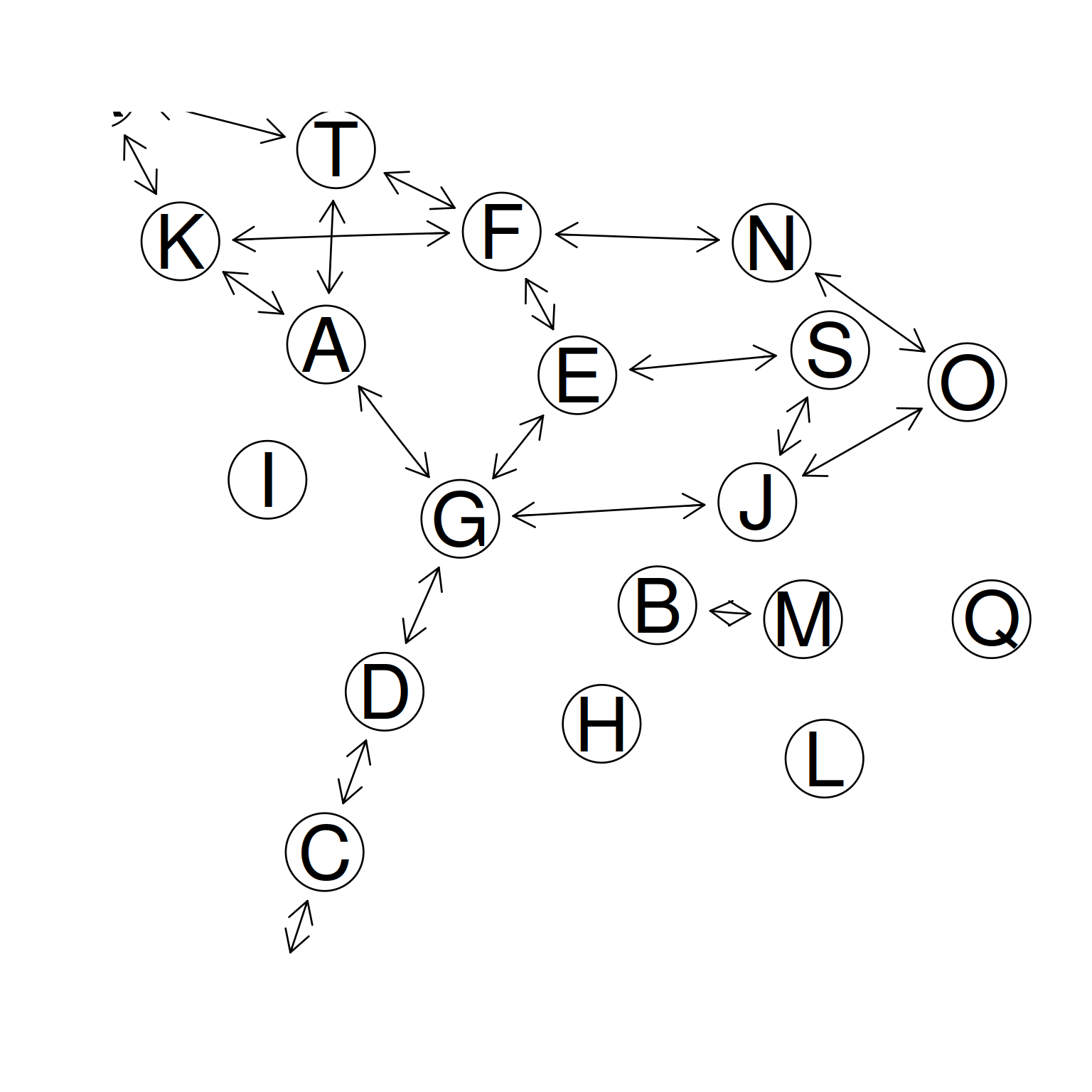
Figure 7.2: GeneNet example
plot(gr2, "fdp")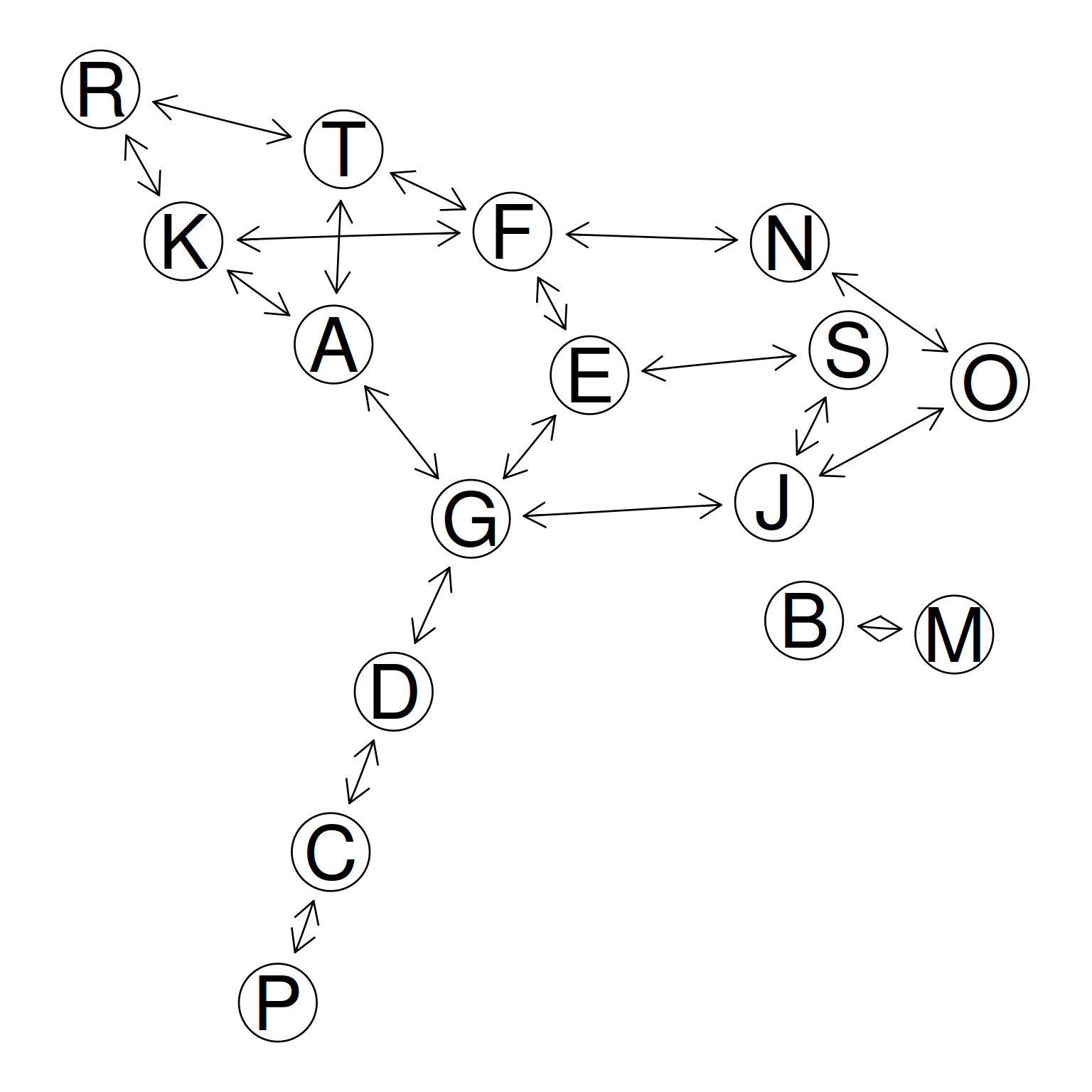
Figure 7.3: GeneNet example
A side-by-side heatmaps
set.seed(123454321)
m <- matrix(runif(2500),50)
r <- cor(m)
g <- as.matrix(r>=0.7)+0
f1 <- ComplexHeatmap::Heatmap(r)
f2 <- ComplexHeatmap::Heatmap(g)
f <- f1+f2
ComplexHeatmap::draw(f)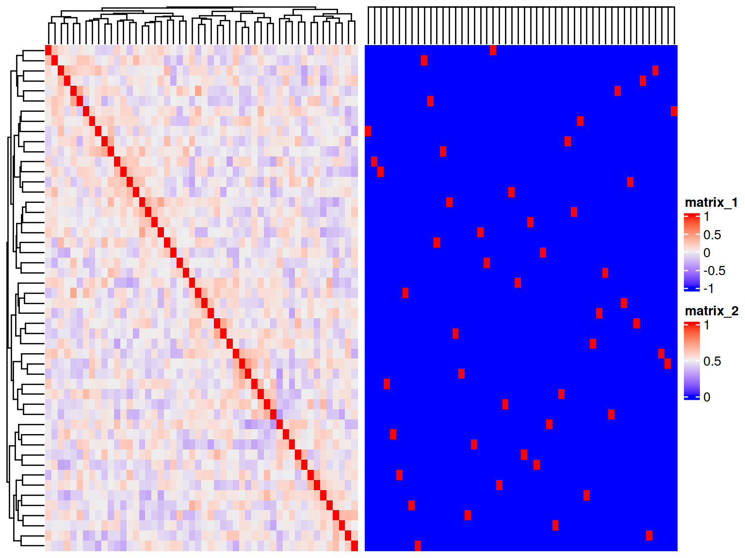
Figure 7.4: Heatmaps
df <- heatmaply::normalize(mtcars)
hm <- heatmaply::heatmaply(df,k_col=5,k_row=5,
                           colors = grDevices::colorRampPalette(RColorBrewer::brewer.pal(3, "RdBu"))(256))
#> Warning: Using `size` aesthetic for lines was deprecated in ggplot2 3.4.0.
#> ℹ Please use `linewidth` instead.
#> ℹ The deprecated feature was likely used in the dendextend package.
#>   Please report the issue at <https://github.com/talgalili/dendextend/issues>.
#> This warning is displayed once per session.
#> Call `lifecycle::last_lifecycle_warnings()` to see where this warning was
#> generated.
htmlwidgets::saveWidget(hm,file="heatmaply.html")
htmltools::tags$iframe(src = "/pQTLtools/articles/heatmaply.html", width = "100%", height = "600px")
and a module analysis with WGCNA,
pwr <- c(1:10, seq(from=12, to=30, by=2))
sft <- WGCNA::pickSoftThreshold(dat, powerVector=pwr, verbose=5)
ADJ <- abs(cor(dat, method="pearson", use="pairwise.complete.obs"))^6
dissADJ <- 1-ADJ
dissTOM <- WGCNA::TOMdist(ADJ)
TOM <- WGCNA::TOMsimilarityFromExpr(dat)
Tree <- hclust(as.dist(1-TOM), method="average")
for(j in pwr)
{
  pam_name <- paste0("pam",j)
  assign(pam_name, cluster::pam(as.dist(dissADJ),j))
  pamTOM_name <- paste0("pamTOM",j)
  assign(pamTOM_name,cluster::pam(as.dist(dissTOM),j))
  tc <- table(get(pam_name)$clustering,get(pamTOM_name)$clustering)
  print(tc)
  print(diag(tc))
}
colorStaticTOM <- as.character(WGCNA::cutreeStaticColor(Tree,cutHeight=.99,minSize=5))
colorDynamicTOM <- WGCNA::labels2colors(cutreeDynamic(Tree,method="tree",minClusterSize=5))
Colors <- data.frame(pamTOM6$clustering,colorStaticTOM,colorDynamicTOM)
WGCNA::plotDendroAndColors(Tree, Colors, dendroLabels=FALSE, hang=0.03, addGuide=TRUE, guideHang=0.05)
meg <- WGCNA::moduleEigengenes(dat, color=1:ncol(dat), softPower=6)
8 Metadata
This section is based on package recount3.
hs <- recount3::available_projects()
dim(subset(hs,file_source=="gtex"))
recount3::annotation_options("human")
blood_rse <- recount3::create_rse(subset(hs,project=="BLOOD"))
S4Vectors::metadata(blood_rse)
SummarizedExperiment::rowRanges(blood_rse)
colnames(SummarizedExperiment::colData(blood_rse))[1:20]
recount3::expand_sra_attributes(blood_rse)
9 Pathway and enrichment analysis
reactome <- graphite::pathways("hsapiens", "reactome")
kegg <- graphite::pathways("hsapiens","kegg")
pharmgkb <- graphite::pathways("hsapiens","pharmgkb")
nodes(kegg[[21]])
#>  [1] "ENTREZID:102724560" "ENTREZID:107080644" "ENTREZID:10993"
#>  [4] "ENTREZID:113675"    "ENTREZID:132158"    "ENTREZID:1610"
#>  [7] "ENTREZID:1738"      "ENTREZID:1757"      "ENTREZID:189"
#> [10] "ENTREZID:211"       "ENTREZID:212"       "ENTREZID:23464"
#> [13] "ENTREZID:2593"      "ENTREZID:26227"     "ENTREZID:2628"
#> [16] "ENTREZID:27232"     "ENTREZID:2731"      "ENTREZID:275"
#> [19] "ENTREZID:29958"     "ENTREZID:29968"     "ENTREZID:441531"
#> [22] "ENTREZID:501"       "ENTREZID:51268"     "ENTREZID:5223"
#> [25] "ENTREZID:5224"      "ENTREZID:55349"     "ENTREZID:5723"
#> [28] "ENTREZID:635"       "ENTREZID:63826"     "ENTREZID:6470"
#> [31] "ENTREZID:6472"      "ENTREZID:64902"     "ENTREZID:669"
#> [34] "ENTREZID:875"       "ENTREZID:9380"      "ENTREZID:1491"
kegg_t2g <- ldply(lapply(kegg, nodes), data.frame)
names(kegg_t2g) <- c("gs_name", "gene_symbol")
VEGF <- subset(kegg_t2g,gs_name=="VEGF signaling pathway")[[2]]
eKEGG <- clusterProfiler::enricher(gene=VEGF, TERM2GENE = kegg_t2g,
                                   universe=,
                                   pAdjustMethod = "BH",
                                   pvalueCutoff = 0.1, qvalueCutoff = 0.05,
                                   minGSSize = 10, maxGSSize = 500)
10 Transcript databases
An overview of annotation is available2.
# columns(org.Hs.eg.db)
# keyref <- keys(org.Hs.eg.db, keytype="ENTREZID")
# symbol_uniprot <- select(org.Hs.eg.db,keys=keyref,columns = c("SYMBOL","UNIPROT"))
# subset(symbol_uniprot,SYMBOL=="MC4R")

x <- EnsDb.Hsapiens.v86
ensembldb::listColumns(x, "protein", skip.keys=TRUE)
#> [1] "tx_id"            "protein_id"       "protein_sequence"
ensembldb::listGenebiotypes(x)
#>  [1] "protein_coding"                     "unitary_pseudogene"
#>  [3] "unprocessed_pseudogene"             "processed_pseudogene"
#>  [5] "processed_transcript"               "transcribed_unprocessed_pseudogene"
#>  [7] "antisense"                          "transcribed_unitary_pseudogene"
#>  [9] "polymorphic_pseudogene"             "lincRNA"
#> [11] "sense_intronic"                     "transcribed_processed_pseudogene"
#> [13] "sense_overlapping"                  "IG_V_pseudogene"
#> [15] "pseudogene"                         "TR_V_gene"
#> [17] "3prime_overlapping_ncRNA"           "IG_V_gene"
#> [19] "bidirectional_promoter_lncRNA"      "snRNA"
#> [21] "miRNA"                              "misc_RNA"
#> [23] "snoRNA"                             "rRNA"
#> [25] "Mt_tRNA"                            "Mt_rRNA"
#> [27] "IG_C_gene"                          "IG_J_gene"
#> [29] "TR_J_gene"                          "TR_C_gene"
#> [31] "TR_V_pseudogene"                    "TR_J_pseudogene"
#> [33] "IG_D_gene"                          "ribozyme"
#> [35] "IG_C_pseudogene"                    "TR_D_gene"
#> [37] "TEC"                                "IG_J_pseudogene"
#> [39] "scRNA"                              "scaRNA"
#> [41] "vaultRNA"                           "sRNA"
#> [43] "macro_lncRNA"                       "non_coding"
#> [45] "IG_pseudogene"                      "LRG_gene"
ensembldb::listTxbiotypes(x)
#>  [1] "protein_coding"                     "processed_transcript"
#>  [3] "nonsense_mediated_decay"            "retained_intron"
#>  [5] "unitary_pseudogene"                 "TEC"
#>  [7] "miRNA"                              "misc_RNA"
#>  [9] "non_stop_decay"                     "unprocessed_pseudogene"
#> [11] "processed_pseudogene"               "transcribed_unprocessed_pseudogene"
#> [13] "lincRNA"                            "antisense"
#> [15] "transcribed_unitary_pseudogene"     "polymorphic_pseudogene"
#> [17] "sense_intronic"                     "transcribed_processed_pseudogene"
#> [19] "sense_overlapping"                  "IG_V_pseudogene"
#> [21] "pseudogene"                         "TR_V_gene"
#> [23] "3prime_overlapping_ncRNA"           "IG_V_gene"
#> [25] "bidirectional_promoter_lncRNA"      "snRNA"
#> [27] "snoRNA"                             "rRNA"
#> [29] "Mt_tRNA"                            "Mt_rRNA"
#> [31] "IG_C_gene"                          "IG_J_gene"
#> [33] "TR_J_gene"                          "TR_C_gene"
#> [35] "TR_V_pseudogene"                    "TR_J_pseudogene"
#> [37] "IG_D_gene"                          "ribozyme"
#> [39] "IG_C_pseudogene"                    "TR_D_gene"
#> [41] "IG_J_pseudogene"                    "scRNA"
#> [43] "scaRNA"                             "vaultRNA"
#> [45] "sRNA"                               "macro_lncRNA"
#> [47] "non_coding"                         "IG_pseudogene"
#> [49] "LRG_gene"
ensembldb::listTables(x)
#> $gene
#> [1] "gene_id"          "gene_name"        "gene_biotype"     "gene_seq_start"
#> [5] "gene_seq_end"     "seq_name"         "seq_strand"       "seq_coord_system"
#> [9] "symbol"
#>
#> $tx
#> [1] "tx_id"            "tx_biotype"       "tx_seq_start"     "tx_seq_end"
#> [5] "tx_cds_seq_start" "tx_cds_seq_end"   "gene_id"          "tx_name"
#>
#> $tx2exon
#> [1] "tx_id"    "exon_id"  "exon_idx"
#>
#> $exon
#> [1] "exon_id"        "exon_seq_start" "exon_seq_end"
#>
#> $chromosome
#> [1] "seq_name"    "seq_length"  "is_circular"
#>
#> $protein
#> [1] "tx_id"            "protein_id"       "protein_sequence"
#>
#> $uniprot
#> [1] "protein_id"           "uniprot_id"           "uniprot_db"
#> [4] "uniprot_mapping_type"
#>
#> $protein_domain
#> [1] "protein_id"            "protein_domain_id"     "protein_domain_source"
#> [4] "interpro_accession"    "prot_dom_start"        "prot_dom_end"
#>
#> $entrezgene
#> [1] "gene_id"  "entrezid"
#>
#> $metadata
#> [1] "name"  "value"
ensembldb::metadata(x)
#>                  name                               value
#> 1             Db type                               EnsDb
#> 2     Type of Gene ID                     Ensembl Gene ID
#> 3  Supporting package                           ensembldb
#> 4       Db created by ensembldb package from Bioconductor
#> 5      script_version                               0.3.0
#> 6       Creation time            Thu May 18 16:32:27 2017
#> 7     ensembl_version                                  86
#> 8        ensembl_host                           localhost
#> 9            Organism                        homo_sapiens
#> 10        taxonomy_id                                9606
#> 11       genome_build                              GRCh38
#> 12    DBSCHEMAVERSION                                 2.0
ensembldb::organism(x)
#> [1] "Homo sapiens"
ensembldb::returnFilterColumns(x)
#> [1] TRUE
ensembldb::seqinfo(x)
#> Seqinfo object with 357 sequences (1 circular) from GRCh38 genome:
#>   seqnames seqlengths isCircular genome
#>   X         156040895      FALSE GRCh38
#>   20         64444167      FALSE GRCh38
#>   1         248956422      FALSE GRCh38
#>   6         170805979      FALSE GRCh38
#>   3         198295559      FALSE GRCh38
#>   ...             ...        ...    ...
#>   LRG_239      114904      FALSE GRCh38
#>   LRG_311      115492      FALSE GRCh38
#>   LRG_721       33396      FALSE GRCh38
#>   LRG_741      231167      FALSE GRCh38
#>   LRG_93        22459      FALSE GRCh38
ensembldb::seqlevels(x)
#>   [1] "1"
#>   [2] "10"
#>   [3] "11"
#>   [4] "12"
#>   [5] "13"
#>   [6] "14"
#>   [7] "15"
#>   [8] "16"
#>   [9] "17"
#>  [10] "18"
#>  [11] "19"
#>  [12] "2"
#>  [13] "20"
#>  [14] "21"
#>  [15] "22"
#>  [16] "3"
#>  [17] "4"
#>  [18] "5"
#>  [19] "6"
#>  [20] "7"
#>  [21] "8"
#>  [22] "9"
#>  [23] "CHR_HG107_PATCH"
#>  [24] "CHR_HG126_PATCH"
#>  [25] "CHR_HG1311_PATCH"
#>  [26] "CHR_HG1342_HG2282_PATCH"
#>  [27] "CHR_HG1362_PATCH"
#>  [28] "CHR_HG142_HG150_NOVEL_TEST"
#>  [29] "CHR_HG151_NOVEL_TEST"
#>  [30] "CHR_HG1651_PATCH"
#>  [31] "CHR_HG1832_PATCH"
#>  [32] "CHR_HG2021_PATCH"
#>  [33] "CHR_HG2022_PATCH"
#>  [34] "CHR_HG2023_PATCH"
#>  [35] "CHR_HG2030_PATCH"
#>  [36] "CHR_HG2058_PATCH"
#>  [37] "CHR_HG2062_PATCH"
#>  [38] "CHR_HG2063_PATCH"
#>  [39] "CHR_HG2066_PATCH"
#>  [40] "CHR_HG2072_PATCH"
#>  [41] "CHR_HG2095_PATCH"
#>  [42] "CHR_HG2104_PATCH"
#>  [43] "CHR_HG2116_PATCH"
#>  [44] "CHR_HG2128_PATCH"
#>  [45] "CHR_HG2191_PATCH"
#>  [46] "CHR_HG2213_PATCH"
#>  [47] "CHR_HG2217_PATCH"
#>  [48] "CHR_HG2232_PATCH"
#>  [49] "CHR_HG2233_PATCH"
#>  [50] "CHR_HG2235_PATCH"
#>  [51] "CHR_HG2239_PATCH"
#>  [52] "CHR_HG2247_PATCH"
#>  [53] "CHR_HG2249_PATCH"
#>  [54] "CHR_HG2288_HG2289_PATCH"
#>  [55] "CHR_HG2290_PATCH"
#>  [56] "CHR_HG2291_PATCH"
#>  [57] "CHR_HG2334_PATCH"
#>  [58] "CHR_HG26_PATCH"
#>  [59] "CHR_HG986_PATCH"
#>  [60] "CHR_HSCHR10_1_CTG1"
#>  [61] "CHR_HSCHR10_1_CTG2"
#>  [62] "CHR_HSCHR10_1_CTG3"
#>  [63] "CHR_HSCHR10_1_CTG4"
#>  [64] "CHR_HSCHR10_1_CTG6"
#>  [65] "CHR_HSCHR11_1_CTG1_2"
#>  [66] "CHR_HSCHR11_1_CTG5"
#>  [67] "CHR_HSCHR11_1_CTG6"
#>  [68] "CHR_HSCHR11_1_CTG7"
#>  [69] "CHR_HSCHR11_1_CTG8"
#>  [70] "CHR_HSCHR11_2_CTG1"
#>  [71] "CHR_HSCHR11_2_CTG1_1"
#>  [72] "CHR_HSCHR11_3_CTG1"
#>  [73] "CHR_HSCHR12_1_CTG1"
#>  [74] "CHR_HSCHR12_1_CTG2_1"
#>  [75] "CHR_HSCHR12_2_CTG1"
#>  [76] "CHR_HSCHR12_2_CTG2"
#>  [77] "CHR_HSCHR12_2_CTG2_1"
#>  [78] "CHR_HSCHR12_3_CTG2"
#>  [79] "CHR_HSCHR12_3_CTG2_1"
#>  [80] "CHR_HSCHR12_4_CTG2"
#>  [81] "CHR_HSCHR12_4_CTG2_1"
#>  [82] "CHR_HSCHR12_5_CTG2"
#>  [83] "CHR_HSCHR12_5_CTG2_1"
#>  [84] "CHR_HSCHR12_6_CTG2_1"
#>  [85] "CHR_HSCHR13_1_CTG1"
#>  [86] "CHR_HSCHR13_1_CTG3"
#>  [87] "CHR_HSCHR13_1_CTG5"
#>  [88] "CHR_HSCHR13_1_CTG8"
#>  [89] "CHR_HSCHR14_1_CTG1"
#>  [90] "CHR_HSCHR14_2_CTG1"
#>  [91] "CHR_HSCHR14_3_CTG1"
#>  [92] "CHR_HSCHR14_7_CTG1"
#>  [93] "CHR_HSCHR15_1_CTG1"
#>  [94] "CHR_HSCHR15_1_CTG3"
#>  [95] "CHR_HSCHR15_1_CTG8"
#>  [96] "CHR_HSCHR15_2_CTG3"
#>  [97] "CHR_HSCHR15_2_CTG8"
#>  [98] "CHR_HSCHR15_3_CTG3"
#>  [99] "CHR_HSCHR15_3_CTG8"
#> [100] "CHR_HSCHR15_4_CTG8"
#> [101] "CHR_HSCHR15_5_CTG8"
#> [102] "CHR_HSCHR15_6_CTG8"
#> [103] "CHR_HSCHR16_1_CTG1"
#> [104] "CHR_HSCHR16_1_CTG3_1"
#> [105] "CHR_HSCHR16_2_CTG3_1"
#> [106] "CHR_HSCHR16_3_CTG1"
#> [107] "CHR_HSCHR16_4_CTG1"
#> [108] "CHR_HSCHR16_4_CTG3_1"
#> [109] "CHR_HSCHR16_5_CTG1"
#> [110] "CHR_HSCHR16_CTG2"
#> [111] "CHR_HSCHR17_10_CTG4"
#> [112] "CHR_HSCHR17_1_CTG1"
#> [113] "CHR_HSCHR17_1_CTG2"
#> [114] "CHR_HSCHR17_1_CTG4"
#> [115] "CHR_HSCHR17_1_CTG5"
#> [116] "CHR_HSCHR17_1_CTG9"
#> [117] "CHR_HSCHR17_2_CTG1"
#> [118] "CHR_HSCHR17_2_CTG2"
#> [119] "CHR_HSCHR17_2_CTG4"
#> [120] "CHR_HSCHR17_2_CTG5"
#> [121] "CHR_HSCHR17_3_CTG2"
#> [122] "CHR_HSCHR17_3_CTG4"
#> [123] "CHR_HSCHR17_4_CTG4"
#> [124] "CHR_HSCHR17_5_CTG4"
#> [125] "CHR_HSCHR17_6_CTG4"
#> [126] "CHR_HSCHR17_7_CTG4"
#> [127] "CHR_HSCHR17_8_CTG4"
#> [128] "CHR_HSCHR17_9_CTG4"
#> [129] "CHR_HSCHR18_1_CTG1_1"
#> [130] "CHR_HSCHR18_1_CTG2_1"
#> [131] "CHR_HSCHR18_2_CTG1_1"
#> [132] "CHR_HSCHR18_2_CTG2"
#> [133] "CHR_HSCHR18_2_CTG2_1"
#> [134] "CHR_HSCHR18_3_CTG2_1"
#> [135] "CHR_HSCHR18_5_CTG1_1"
#> [136] "CHR_HSCHR18_ALT21_CTG2_1"
#> [137] "CHR_HSCHR18_ALT2_CTG2_1"
#> [138] "CHR_HSCHR19KIR_ABC08_A1_HAP_CTG3_1"
#> [139] "CHR_HSCHR19KIR_ABC08_AB_HAP_C_P_CTG3_1"
#> [140] "CHR_HSCHR19KIR_ABC08_AB_HAP_T_P_CTG3_1"
#> [141] "CHR_HSCHR19KIR_FH05_A_HAP_CTG3_1"
#> [142] "CHR_HSCHR19KIR_FH05_B_HAP_CTG3_1"
#> [143] "CHR_HSCHR19KIR_FH06_A_HAP_CTG3_1"
#> [144] "CHR_HSCHR19KIR_FH06_BA1_HAP_CTG3_1"
#> [145] "CHR_HSCHR19KIR_FH08_A_HAP_CTG3_1"
#> [146] "CHR_HSCHR19KIR_FH08_BAX_HAP_CTG3_1"
#> [147] "CHR_HSCHR19KIR_FH13_A_HAP_CTG3_1"
#> [148] "CHR_HSCHR19KIR_FH13_BA2_HAP_CTG3_1"
#> [149] "CHR_HSCHR19KIR_FH15_A_HAP_CTG3_1"
#> [150] "CHR_HSCHR19KIR_FH15_B_HAP_CTG3_1"
#> [151] "CHR_HSCHR19KIR_G085_A_HAP_CTG3_1"
#> [152] "CHR_HSCHR19KIR_G085_BA1_HAP_CTG3_1"
#> [153] "CHR_HSCHR19KIR_G248_A_HAP_CTG3_1"
#> [154] "CHR_HSCHR19KIR_G248_BA2_HAP_CTG3_1"
#> [155] "CHR_HSCHR19KIR_GRC212_AB_HAP_CTG3_1"
#> [156] "CHR_HSCHR19KIR_GRC212_BA1_HAP_CTG3_1"
#> [157] "CHR_HSCHR19KIR_LUCE_A_HAP_CTG3_1"
#> [158] "CHR_HSCHR19KIR_LUCE_BDEL_HAP_CTG3_1"
#> [159] "CHR_HSCHR19KIR_RP5_B_HAP_CTG3_1"
#> [160] "CHR_HSCHR19KIR_RSH_A_HAP_CTG3_1"
#> [161] "CHR_HSCHR19KIR_RSH_BA2_HAP_CTG3_1"
#> [162] "CHR_HSCHR19KIR_T7526_A_HAP_CTG3_1"
#> [163] "CHR_HSCHR19KIR_T7526_BDEL_HAP_CTG3_1"
#> [164] "CHR_HSCHR19LRC_COX1_CTG3_1"
#> [165] "CHR_HSCHR19LRC_COX2_CTG3_1"
#> [166] "CHR_HSCHR19LRC_LRC_I_CTG3_1"
#> [167] "CHR_HSCHR19LRC_LRC_J_CTG3_1"
#> [168] "CHR_HSCHR19LRC_LRC_S_CTG3_1"
#> [169] "CHR_HSCHR19LRC_LRC_T_CTG3_1"
#> [170] "CHR_HSCHR19LRC_PGF1_CTG3_1"
#> [171] "CHR_HSCHR19LRC_PGF2_CTG3_1"
#> [172] "CHR_HSCHR19_1_CTG2"
#> [173] "CHR_HSCHR19_1_CTG3_1"
#> [174] "CHR_HSCHR19_2_CTG2"
#> [175] "CHR_HSCHR19_2_CTG3_1"
#> [176] "CHR_HSCHR19_3_CTG2"
#> [177] "CHR_HSCHR19_3_CTG3_1"
#> [178] "CHR_HSCHR19_4_CTG2"
#> [179] "CHR_HSCHR19_4_CTG3_1"
#> [180] "CHR_HSCHR19_5_CTG2"
#> [181] "CHR_HSCHR1_1_CTG11"
#> [182] "CHR_HSCHR1_1_CTG3"
#> [183] "CHR_HSCHR1_1_CTG31"
#> [184] "CHR_HSCHR1_1_CTG32_1"
#> [185] "CHR_HSCHR1_2_CTG3"
#> [186] "CHR_HSCHR1_2_CTG31"
#> [187] "CHR_HSCHR1_2_CTG32_1"
#> [188] "CHR_HSCHR1_3_CTG3"
#> [189] "CHR_HSCHR1_3_CTG31"
#> [190] "CHR_HSCHR1_3_CTG32_1"
#> [191] "CHR_HSCHR1_4_CTG3"
#> [192] "CHR_HSCHR1_4_CTG31"
#> [193] "CHR_HSCHR1_5_CTG3"
#> [194] "CHR_HSCHR1_5_CTG32_1"
#> [195] "CHR_HSCHR1_ALT2_1_CTG32_1"
#> [196] "CHR_HSCHR20_1_CTG1"
#> [197] "CHR_HSCHR20_1_CTG2"
#> [198] "CHR_HSCHR20_1_CTG3"
#> [199] "CHR_HSCHR20_1_CTG4"
#> [200] "CHR_HSCHR21_2_CTG1_1"
#> [201] "CHR_HSCHR21_3_CTG1_1"
#> [202] "CHR_HSCHR21_4_CTG1_1"
#> [203] "CHR_HSCHR21_5_CTG2"
#> [204] "CHR_HSCHR21_6_CTG1_1"
#> [205] "CHR_HSCHR21_8_CTG1_1"
#> [206] "CHR_HSCHR22_1_CTG1"
#> [207] "CHR_HSCHR22_1_CTG2"
#> [208] "CHR_HSCHR22_1_CTG3"
#> [209] "CHR_HSCHR22_1_CTG4"
#> [210] "CHR_HSCHR22_1_CTG5"
#> [211] "CHR_HSCHR22_1_CTG6"
#> [212] "CHR_HSCHR22_1_CTG7"
#> [213] "CHR_HSCHR22_2_CTG1"
#> [214] "CHR_HSCHR22_3_CTG1"
#> [215] "CHR_HSCHR22_4_CTG1"
#> [216] "CHR_HSCHR22_5_CTG1"
#> [217] "CHR_HSCHR22_6_CTG1"
#> [218] "CHR_HSCHR22_7_CTG1"
#> [219] "CHR_HSCHR22_8_CTG1"
#> [220] "CHR_HSCHR2_1_CTG1"
#> [221] "CHR_HSCHR2_1_CTG15"
#> [222] "CHR_HSCHR2_1_CTG5"
#> [223] "CHR_HSCHR2_1_CTG7"
#> [224] "CHR_HSCHR2_1_CTG7_2"
#> [225] "CHR_HSCHR2_2_CTG1"
#> [226] "CHR_HSCHR2_2_CTG15"
#> [227] "CHR_HSCHR2_2_CTG7"
#> [228] "CHR_HSCHR2_2_CTG7_2"
#> [229] "CHR_HSCHR2_3_CTG1"
#> [230] "CHR_HSCHR2_3_CTG15"
#> [231] "CHR_HSCHR2_3_CTG7_2"
#> [232] "CHR_HSCHR2_4_CTG1"
#> [233] "CHR_HSCHR2_6_CTG7_2"
#> [234] "CHR_HSCHR3_1_CTG1"
#> [235] "CHR_HSCHR3_1_CTG2_1"
#> [236] "CHR_HSCHR3_1_CTG3"
#> [237] "CHR_HSCHR3_2_CTG2_1"
#> [238] "CHR_HSCHR3_2_CTG3"
#> [239] "CHR_HSCHR3_3_CTG1"
#> [240] "CHR_HSCHR3_3_CTG3"
#> [241] "CHR_HSCHR3_4_CTG2_1"
#> [242] "CHR_HSCHR3_4_CTG3"
#> [243] "CHR_HSCHR3_5_CTG2_1"
#> [244] "CHR_HSCHR3_5_CTG3"
#> [245] "CHR_HSCHR3_6_CTG3"
#> [246] "CHR_HSCHR3_7_CTG3"
#> [247] "CHR_HSCHR3_8_CTG3"
#> [248] "CHR_HSCHR3_9_CTG3"
#> [249] "CHR_HSCHR4_11_CTG12"
#> [250] "CHR_HSCHR4_1_CTG12"
#> [251] "CHR_HSCHR4_1_CTG4"
#> [252] "CHR_HSCHR4_1_CTG6"
#> [253] "CHR_HSCHR4_1_CTG9"
#> [254] "CHR_HSCHR4_2_CTG12"
#> [255] "CHR_HSCHR4_2_CTG4"
#> [256] "CHR_HSCHR4_3_CTG12"
#> [257] "CHR_HSCHR4_4_CTG12"
#> [258] "CHR_HSCHR4_5_CTG12"
#> [259] "CHR_HSCHR4_6_CTG12"
#> [260] "CHR_HSCHR4_7_CTG12"
#> [261] "CHR_HSCHR4_8_CTG12"
#> [262] "CHR_HSCHR4_9_CTG12"
#> [263] "CHR_HSCHR5_1_CTG1"
#> [264] "CHR_HSCHR5_1_CTG1_1"
#> [265] "CHR_HSCHR5_1_CTG5"
#> [266] "CHR_HSCHR5_2_CTG1"
#> [267] "CHR_HSCHR5_2_CTG1_1"
#> [268] "CHR_HSCHR5_2_CTG5"
#> [269] "CHR_HSCHR5_3_CTG1"
#> [270] "CHR_HSCHR5_3_CTG5"
#> [271] "CHR_HSCHR5_4_CTG1"
#> [272] "CHR_HSCHR5_4_CTG1_1"
#> [273] "CHR_HSCHR5_5_CTG1"
#> [274] "CHR_HSCHR5_6_CTG1"
#> [275] "CHR_HSCHR5_7_CTG1"
#> [276] "CHR_HSCHR6_1_CTG10"
#> [277] "CHR_HSCHR6_1_CTG2"
#> [278] "CHR_HSCHR6_1_CTG3"
#> [279] "CHR_HSCHR6_1_CTG4"
#> [280] "CHR_HSCHR6_1_CTG5"
#> [281] "CHR_HSCHR6_1_CTG6"
#> [282] "CHR_HSCHR6_1_CTG7"
#> [283] "CHR_HSCHR6_1_CTG8"
#> [284] "CHR_HSCHR6_1_CTG9"
#> [285] "CHR_HSCHR6_8_CTG1"
#> [286] "CHR_HSCHR6_MHC_APD_CTG1"
#> [287] "CHR_HSCHR6_MHC_COX_CTG1"
#> [288] "CHR_HSCHR6_MHC_DBB_CTG1"
#> [289] "CHR_HSCHR6_MHC_MANN_CTG1"
#> [290] "CHR_HSCHR6_MHC_MCF_CTG1"
#> [291] "CHR_HSCHR6_MHC_QBL_CTG1"
#> [292] "CHR_HSCHR6_MHC_SSTO_CTG1"
#> [293] "CHR_HSCHR7_1_CTG1"
#> [294] "CHR_HSCHR7_1_CTG4_4"
#> [295] "CHR_HSCHR7_1_CTG6"
#> [296] "CHR_HSCHR7_1_CTG7"
#> [297] "CHR_HSCHR7_2_CTG1"
#> [298] "CHR_HSCHR7_2_CTG4_4"
#> [299] "CHR_HSCHR7_2_CTG6"
#> [300] "CHR_HSCHR7_2_CTG7"
#> [301] "CHR_HSCHR7_3_CTG6"
#> [302] "CHR_HSCHR8_1_CTG1"
#> [303] "CHR_HSCHR8_1_CTG6"
#> [304] "CHR_HSCHR8_1_CTG7"
#> [305] "CHR_HSCHR8_2_CTG1"
#> [306] "CHR_HSCHR8_2_CTG7"
#> [307] "CHR_HSCHR8_3_CTG1"
#> [308] "CHR_HSCHR8_3_CTG7"
#> [309] "CHR_HSCHR8_4_CTG1"
#> [310] "CHR_HSCHR8_4_CTG7"
#> [311] "CHR_HSCHR8_5_CTG1"
#> [312] "CHR_HSCHR8_5_CTG7"
#> [313] "CHR_HSCHR8_6_CTG1"
#> [314] "CHR_HSCHR8_7_CTG1"
#> [315] "CHR_HSCHR8_8_CTG1"
#> [316] "CHR_HSCHR8_9_CTG1"
#> [317] "CHR_HSCHR9_1_CTG1"
#> [318] "CHR_HSCHR9_1_CTG2"
#> [319] "CHR_HSCHR9_1_CTG3"
#> [320] "CHR_HSCHR9_1_CTG4"
#> [321] "CHR_HSCHR9_1_CTG5"
#> [322] "CHR_HSCHR9_1_CTG6"
#> [323] "CHR_HSCHRX_1_CTG3"
#> [324] "CHR_HSCHRX_2_CTG12"
#> [325] "CHR_HSCHRX_2_CTG3"
#> [326] "GL000009.2"
#> [327] "GL000194.1"
#> [328] "GL000195.1"
#> [329] "GL000205.2"
#> [330] "GL000213.1"
#> [331] "GL000216.2"
#> [332] "GL000218.1"
#> [333] "GL000219.1"
#> [334] "GL000220.1"
#> [335] "GL000225.1"
#> [336] "KI270442.1"
#> [337] "KI270711.1"
#> [338] "KI270713.1"
#> [339] "KI270721.1"
#> [340] "KI270726.1"
#> [341] "KI270727.1"
#> [342] "KI270728.1"
#> [343] "KI270731.1"
#> [344] "KI270733.1"
#> [345] "KI270734.1"
#> [346] "KI270744.1"
#> [347] "KI270750.1"
#> [348] "LRG_183"
#> [349] "LRG_187"
#> [350] "LRG_239"
#> [351] "LRG_311"
#> [352] "LRG_721"
#> [353] "LRG_741"
#> [354] "LRG_93"
#> [355] "MT"
#> [356] "X"
#> [357] "Y"
ensembldb::updateEnsDb(x)
#> EnsDb for Ensembl:
#> |Backend: SQLite
#> |Db type: EnsDb
#> |Type of Gene ID: Ensembl Gene ID
#> |Supporting package: ensembldb
#> |Db created by: ensembldb package from Bioconductor
#> |script_version: 0.3.0
#> |Creation time: Thu May 18 16:32:27 2017
#> |ensembl_version: 86
#> |ensembl_host: localhost
#> |Organism: homo_sapiens
#> |taxonomy_id: 9606
#> |genome_build: GRCh38
#> |DBSCHEMAVERSION: 2.0
#> | No. of genes: 63970.
#> | No. of transcripts: 216741.
#> |Protein data available.

ensembldb::genes(x, columns=c("gene_name"),
             filter=list(SeqNameFilter("X"), AnnotationFilter::GeneBiotypeFilter("protein_coding")))
#> GRanges object with 841 ranges and 3 metadata columns:
#>                   seqnames              ranges strand |   gene_name
#>                      <Rle>           <IRanges>  <Rle> | <character>
#>   ENSG00000182378        X       276322-303356      + |      PLCXD1
#>   ENSG00000178605        X       304529-318819      - |      GTPBP6
#>   ENSG00000167393        X       333963-386955      - |     PPP2R3B
#>   ENSG00000185960        X       624344-659411      + |        SHOX
#>   ENSG00000205755        X     1187549-1212750      - |       CRLF2
#>               ...      ...                 ...    ... .         ...
#>   ENSG00000277745        X 155459415-155460005      - |      H2AFB3
#>   ENSG00000185973        X 155490115-155669944      - |       TMLHE
#>   ENSG00000168939        X 155767812-155782459      + |       SPRY3
#>   ENSG00000124333        X 155881293-155943769      + |       VAMP7
#>   ENSG00000124334        X 155997581-156010817      + |        IL9R
#>                         gene_id  gene_biotype
#>                     <character>   <character>
#>   ENSG00000182378 ENSG000001... protein_co...
#>   ENSG00000178605 ENSG000001... protein_co...
#>   ENSG00000167393 ENSG000001... protein_co...
#>   ENSG00000185960 ENSG000001... protein_co...
#>   ENSG00000205755 ENSG000002... protein_co...
#>               ...           ...           ...
#>   ENSG00000277745 ENSG000002... protein_co...
#>   ENSG00000185973 ENSG000001... protein_co...
#>   ENSG00000168939 ENSG000001... protein_co...
#>   ENSG00000124333 ENSG000001... protein_co...
#>   ENSG00000124334 ENSG000001... protein_co...
#>   -------
#>   seqinfo: 1 sequence from GRCh38 genome
ensembldb ::transcripts(x, columns=ensembldb::listColumns(x, "tx"),
                        filter = AnnotationFilter::AnnotationFilterList(), order.type = "asc", return.type = "GRanges")
#> GRanges object with 216741 ranges and 6 metadata columns:
#>                   seqnames            ranges strand |         tx_id
#>                      <Rle>         <IRanges>  <Rle> |   <character>
#>   ENST00000456328        1       11869-14409      + | ENST000004...
#>   ENST00000450305        1       12010-13670      + | ENST000004...
#>   ENST00000488147        1       14404-29570      - | ENST000004...
#>   ENST00000619216        1       17369-17436      - | ENST000006...
#>   ENST00000473358        1       29554-31097      + | ENST000004...
#>               ...      ...               ...    ... .           ...
#>   ENST00000420810        Y 26549425-26549743      + | ENST000004...
#>   ENST00000456738        Y 26586642-26591601      - | ENST000004...
#>   ENST00000435945        Y 26594851-26634652      - | ENST000004...
#>   ENST00000435741        Y 26626520-26627159      - | ENST000004...
#>   ENST00000431853        Y 56855244-56855488      + | ENST000004...
#>                      tx_biotype tx_cds_seq_start tx_cds_seq_end       gene_id
#>                     <character>        <integer>      <integer>   <character>
#>   ENST00000456328 processed_...             <NA>           <NA> ENSG000002...
#>   ENST00000450305 transcribe...             <NA>           <NA> ENSG000002...
#>   ENST00000488147 unprocesse...             <NA>           <NA> ENSG000002...
#>   ENST00000619216         miRNA             <NA>           <NA> ENSG000002...
#>   ENST00000473358       lincRNA             <NA>           <NA> ENSG000002...
#>               ...           ...              ...            ...           ...
#>   ENST00000420810 processed_...             <NA>           <NA> ENSG000002...
#>   ENST00000456738 unprocesse...             <NA>           <NA> ENSG000002...
#>   ENST00000435945 unprocesse...             <NA>           <NA> ENSG000002...
#>   ENST00000435741 processed_...             <NA>           <NA> ENSG000002...
#>   ENST00000431853 processed_...             <NA>           <NA> ENSG000002...
#>                         tx_name
#>                     <character>
#>   ENST00000456328 ENST000004...
#>   ENST00000450305 ENST000004...
#>   ENST00000488147 ENST000004...
#>   ENST00000619216 ENST000006...
#>   ENST00000473358 ENST000004...
#>               ...           ...
#>   ENST00000420810 ENST000004...
#>   ENST00000456738 ENST000004...
#>   ENST00000435945 ENST000004...
#>   ENST00000435741 ENST000004...
#>   ENST00000431853 ENST000004...
#>   -------
#>   seqinfo: 357 sequences (1 circular) from GRCh38 genome

#txdbEnsemblGRCh38 <- GenomicFeatures::makeTxDbFromEnsembl(organism="Homo sapiens", release=98)
#txdb <- as.list(txdbEnsemblGRCh38)
#lapply(txdb,head)
11 Spectrum data analysis
This section collects notes on peptide/protein analysis, especially with respect to spectrum data.
11.1 Peptide sequence
Here is an example for PROC_HUMAN, which is handled by the Biostrings package,
fasta_file_path <- 'https://rest.uniprot.org/uniprotkb/P04070.fasta'
fasta_sequences <- Biostrings::readAAStringSet(fasta_file_path, format = "fasta")
AA_sequence <- fasta_sequences[[1]]
cat("Sequence:", toString(AA_sequence), "\n")
iso_442688365 <- 'TDGEGALSEPSATVTIEELAAPPPPVLMHHGESSQVLHPGNK'
match_position <- regexpr(iso_442688365, AA_sequence)
match_position
mp <- matchPattern(iso_442688365,AA_sequence)
mp
load(system.file("tests","PROC.rda",package="pQTLtools"))
pQTLtools::peptideAssociationPlot(protein,cistrans)
#> Joining with `by = join_by(Modified.Peptide.Sequence)`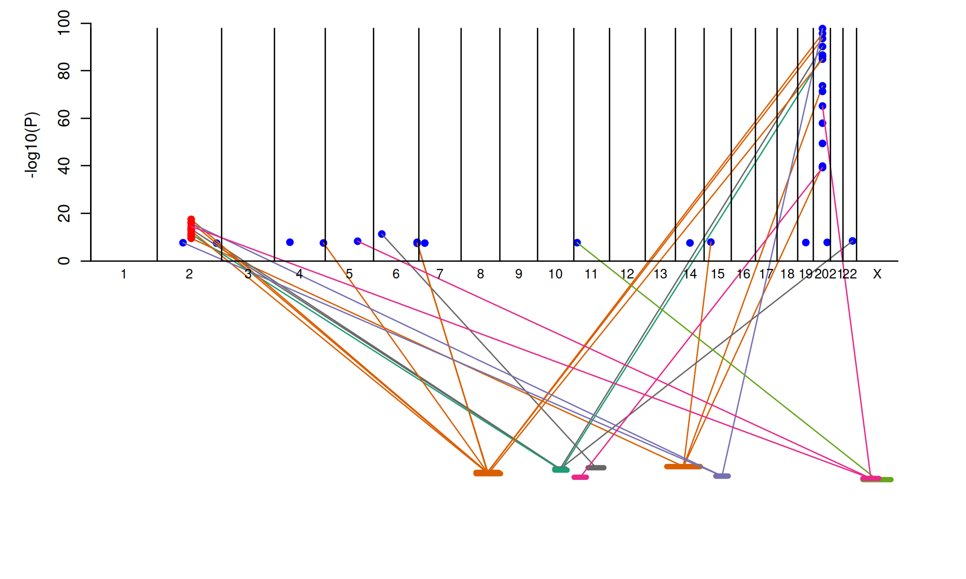
Figure 11.1: peptide association plot
11.2 Spectrum data analysis
11.2.1 Setup
The .raw files can be handled by rawrr package nevertheless it requires necessary files,
library(rawrr)
if (isFALSE(rawrr::.checkDllInMonoPath())){
   rawrr::installRawFileReaderDLLs()
}
if (isFALSE(file.exists(rawrr:::.rawrrAssembly()))){
   rawrr::installRawrrExe()
}
11.2.2 List of.raw files
Based on a real project, the following is an example of listing/generating multiple .raw from .zip files
# ZWK .raw data
spectra_ZWK <- "~/Caprion/pre_qc_data/spectral_library_ZWK"
raw_files <- list.files(spectra_ZWK, pattern = "\\.raw$", full.names = TRUE)
## collectively
suppressMessages(library(MsBackendRawFileReader))
ZWK <- Spectra::backendInitialize(MsBackendRawFileReader::MsBackendRawFileReader(),
       files = raw_files)
class(ZWK)
methods(class=class(ZWK))
Spectra(ZWK)
spectraData(ZWK)
ZWK
ZWKvars <- ZWK |> Spectra::spectraVariables()
ZWKdata <- ZWK |> Spectra::spectraData()
dim(ZWKdata)
# rows with >=1 non-NA value in the columns with prefix "precursor"
precursor <- apply(ZWKdata[grep("precursor",ZWKvars)], 1, function(x) any(!is.na(x)))
ZWKdata_filtered <- ZWKdata[precursor, ]
save(ZWK,file="~/Caprion/analysis/work/ZWK.rda")

# ZYQ/UDP
library(utils)
spectra <- "~/Caprion/pre_qc_data/spectra"
zip_files <- dir(spectra, recursive = TRUE, full.names=TRUE)
work_dir <- "~/Caprion/analysis/work"
for (zip_file in zip_files) unzip(zip_file, exdir=work_dir)
ZYQ_UDP <- Spectra::backendInitialize(MsBackendRawFileReader::MsBackendRawFileReader(),
           files = dir(work_dir,patt="raw",full.names=TRUE))
class(ZYQ_UDP)
ZYQ_UDP
ZYQ_UDP |> Spectra::spectraVariables()
save(ZYQ_UDP,file="~/Caprion/analysis/work/ZYQ_UDP.rda")
11.2.3 Usage
Various facilities are shown below.
# various files
d <- "/rds/project/rds-zuZwCZMsS0w/Caprion_proteomics/analysis/crux"
f <- file.path(d,"szwk901104i19801xms1.mzML")
x <- file.path(d,"szwk901104i19801xms1.mzXML")
g <- file.path(d,"szwk901104i19801xms1.mgf")
r <- file.path(d,"szwk901104i19801xms1.rda")
z <- file.path(d,"szwk901104i19801xms1.mzML.gz")

# mzML
mz <- mzR::openMSfile(f)
header_info <- mzR::header(mz)
table(header_info$msLevel)
peak_data <- mzR::peaks(mz)
spec <- mzR::spectra(mz)
class(spec)
length(spec)
lapply(spec,head,3)
methods(class="mzRpwiz")
mzR::close(mz)

mz <- mzR::openMSfile(z, backend = "pwiz")
mz
nChrom(mz)
head(tic(mz))
head(chromatogram(mz, 1L)) ## same as tic(x)
str(chromatogram(mz))
head(peaks(mz, scan=4))

# MSnbase
mzXML <- MSnbase::readMSData(x)
mgf <- MSnbase::readMgfData(g)
save(mzXML,mgf,file=r)

MSnbase::extractSpectraData(mzXML)
MSnbase::hasSpectra(z)
MSnbase::hasChromatograms(z)
MSnbase::plot2d(mzXML,z="peaks.count")
MSnbase::plotDensity(mzXML,z="precursor.mz")

MSnbase::extractSpectraData(mgf)
methods(class="MSpectra")
MSnbase::mz(mgf)
MSnbase::intensity(mgf)
MSnbase::rtime(mgf)
MSnbase::precursorMz(mgf)
MSnbase::precursorCharge(mgf)
MSnbase::precScanNum(mgf)
MSnbase::precursorIntensity(mgf)
MSnbase::acquisitionNum(mgf)
MSnbase::scanIndex(mgf)
MSnbase::peaksCount(mgf)
MSnbase::msLevel(mgf)
MSnbase::tic(mgf)
MSnbase::ionCount(mgf)
MSnbase::collisionEnergy(mgf)
MSnbase::fromFile(mgf)
MSnbase::polarity(mgf)
MSnbase::smoothed(mgf)
MSnbase::centroided(mgf)
MSnbase::isCentroided(mgf)
MSnbase::writeMgfData(mgf, con = "spectra.mgf", COM = NULL, TITLE = NULL)
MSnbase::removePeaks(mgf, t, msLevel., ...)
MSnbase::filterMsLevel(mgf, msLevel=2)
MSnbase::as.ExpressionSet(mgf)

# This turned to be really slow!
sp_list <- lapply(seq_along(mgf), function(i) {
  intensity_i <- MSnbase::intensity(mgf)[[i]]
  mz_i <- MSnbase::mz(mgf)[[i]]
  centroided_i <- MSnbase::centroided(mgf)[[i]]
  return(new("Spectrum1", intensity = intensity_i, mz = mz_i, centroided = centroided_i))
})
sp1 <- do.call(rbind, sp_list)
# only the first one is more manageable
sp1 <- new("Spectrum1",intensity=MSnbase::intensity(mgf)[[1]],mz=MSnbase::mz(mgf)[[1]],centroided=MSnbase::centroided(mgf)[[1]])
sp2 <- MSnbase::pickPeaks(sp1)
MSnbase::intensity(sp2)
plot(MSnbase::mz(sp1),MSnbase::intensity(sp1),type="h")
## Without m/z refinement
points(MSnbase::mz(sp2), MSnbase::intensity(sp2), col = "darkgrey")
## Using k = 1, closest signals
sp3 <- MSnbase::pickPeaks(sp1, refineMz = "kNeighbors", k = 1)
points(MSnbase::mz(sp3), MSnbase::intensity(sp3), col = "green", type = "h")
## Using descendPeak requiring at least 50% or the centroid's intensity
sp4 <- MSnbase::pickPeaks(sp1, refineMz = "descendPeak", signalPercentage = 50)
points(MSnbase::mz(sp4), MSnbase::intensity(sp4), col = "red", type = "h")

# CAMERA
xs   <- CAMERA::xcmsSet(f, method="centWave", ppm=30, peakwidth=c(5,10))
an   <- CAMERA::xsAnnotate(xs)
an   <- CAMERA::groupFWHM(an)
#For one group
peaklist <- CAMERA::getpspectra(an, 1)
#For two groups
peaklist <- CAMERA::getpspectra(an, c(1,2))

# Spectra
suppressMessages(library(Spectra))
sp <- Spectra::Spectra(z)
head(sp)
table(sp$msLevel)
d <- Spectra::computeMzDeltas(sp[1:1000])
Spectra::plotMzDelta(d)

# protViz
protViz::fragmentIon("TFVLNFIK")
esd <- MSnbase::extractSpectraData(mgf)
op <- par(mfrow=c(2,1))
ms <- function(i) with(esd[i,],list(title=TITLE,rtinseconds=RTINSECONDS,pepmass=PEPMASS,charge=CHARGE,
                                    mZ=MSnbase::mz(mgf[[i]]),intensity=MSnbase::intensity(mgf[[i]])))
protViz::peakplot("TAFDEAIAELDTLNEESYK", ms(1))
protViz::peakplot("TAFDEAIAELDTLSEESYK", ms(2))
par(op)
load("~/Caprion/pilot/ZWK.rda")
peptides <- subset(mapping_ZWK,Protein=="PROC_HUMAN")[["Modified.Peptide.Sequence"]] |> unique()
pim <- protViz::parentIonMass(peptides)
fi <- protViz::fragmentIon(peptides)
df <- as.data.frame(fi)
op <- par(mfrow=c(3,1))
for (i in 1:length(peptides)){
    plot(0, 0,
    xlab='m/Z',
    ylab='',
    xlim=range(c(fi[[i]]$b,fi[[i]]$y)),
    ylim=c(0,1),
    type='n',
    axes=FALSE,
    sub=paste(peptides[i], "/", pim[i], "Da"));
    box()
    axis(1, fi[[i]]$b, round(fi[[i]]$b,1), las=2)
    axis(1, fi[[i]]$y, round(fi[[i]]$y,1), las=2)

    pepSeq<-strsplit(peptides[i], "")
    axis(3,fi[[i]]$b, paste("b", row.names(fi[[i]]),sep=''),las=2)
    axis(3,fi[[i]]$y, paste("y", row.names(fi[[i]]),sep=''),las=2)

    text(fi[[i]]$b, rep(0.3, nchar(peptides[i])),
    pepSeq[[1]],pos=3,cex=4, lwd=4, col="#aaaaaaaa")

    abline(v=fi[[i]]$b, col='red')
    abline(v=fi[[i]]$y, col='blue',lwd=2)
}
par(op)

# MSstats
head(SRMRawData)
QuantData <- MSstats::dataProcess(SRMRawData, use_log_file = FALSE)
quant <- MSstats::dataProcess(SRMRawData,
                              normalization = "equalizeMedians",
                              summaryMethod = "TMP",
                              censoredInt = "NA",
                              MBimpute = TRUE,
                              maxQuantileforCensored = 0.999,
                              logTrans=2,
                              use_log_file=FALSE,
                              numberOfCores=5)
names(quant)MSstats3 takes output from other data-processing pipelines.
13 Bioconductor/CRAN packages
| Package | Description |
|---|---|
| Bioconductor | |
| AnnotationDbi | AnnotationDb objects and their progeny, methods etc. |
| Biobase | Base functions for Bioconductor |
| Biostrings | Efficient manipulation of biological strings |
| CAMERA | Collection of annotation related methods |
| clusterProfiler | Functional profiles for genes and gene clusters |
| ComplexHeatmap | Make complex heatmaps |
| DESSeq2 | Differential gene expression analysis based on the negative binomial distribution |
| edgeR | Empirical analysis of digital gene expression |
| EnsDb.Hsapiens.v86 | Exposes an annotation databases generated from Ensembl |
| ensembldb | Retrieve annotation data from an Ensembl based package |
| FlowSorted.DLPFC.450k | Illumina HumanMethylation data on sorted frontal cortex cell populations |
| graphite | GRAPH Interaction from pathway topological environment |
| IlluminaHumanMethylation450kmanifest | Annotation for Illumina’s 450k methylation arrays |
| INSPEcT | Quantification of the intronic and exonic gene features and the post-transcriptional regulation analysis |
| MSnbase | Base Functions and Classes for Mass Spectrometry and Proteomics |
| MSstats | Protein Significance Analysis in DDA, SRM and DIA Proteomics |
| mzR | parser for netCDF, mzXML and mzML and mzIdentML files |
| org.Hs.eg.db | Conversion of Entrez ID – gene symbols |
| OUTRIDER | OUTlier in RNA-Seq fInDER |
| Pi | Priority index, leveraging genetic evidence to prioritise drug targets at the gene and pathway level |
| quantro | A test for when to use quantile normalisation |
| rawrr | Direct Access to Orbitrap Data and Beyond |
| recount3 | Interface to uniformly processed RNA-seq data |
| Rgraphiz | Interfaces R with the AT&T graphviz library for plotting R graph objects from the graph package |
| Spectra | Spectra Infrastructure for Mass Spectrometry |
| sva | Surrogate Variable Analysis |
| TxDb.Hsapiens.UCSC.hg38.knownGene | Annotation of the human genome |
| CRAN | |
| doParallel | Foreach Parallel Adaptor for the ‘parallel’ Package |
| GeneNet | Modeling and Inferring Gene Networks |
| ggplot2 | Data Visualisations Using the grammar of graphics |
| heatmaply | Interactive Cluster Heat Maps Using plotly and ggplot2
|
| pheatmap | results visualisation |
| plyr | Splitting, applying and combining data |
| protViz | Foreach Parallel Adaptor for the ‘parallel’ Package |
| RColorBrewer | ColorBrewer Palettes |
| WGCNA | Weighted correlation network analysis |