ExpressionSet/SummarizedExperiment usage • pQTLtools

es_pkgs <- c("Biobase", "arrayQualityMetrics", "dplyr", "knitr", "mclust", "pQTLtools", "rgl", "scatterplot3d")
se_pkgs <- c("BiocGenerics","GenomicRanges","IRanges","MsCoreUtils","S4Vectors","SummarizedExperiment")
pkgs <- c(es_pkgs,se_pkgs)
for (p in pkgs) if (length(grep(paste("^package:", p, "$", sep=""), search())) == 0) {
    if (!requireNamespace(p)) warning(paste0("This vignette needs package `", p, "'; please install"))
}
invisible(suppressMessages(lapply(pkgs, require, character.only = TRUE)))

1 ExpressionSet

We start with Bioconductor/Biobase’s ExpressionSet example and finish with a real application.

dataDirectory <- system.file("extdata", package="Biobase")
exprsFile <- file.path(dataDirectory, "exprsData.txt")
exprs <- as.matrix(read.table(exprsFile, header=TRUE, sep="\t", row.names=1, as.is=TRUE))
pDataFile <- file.path(dataDirectory, "pData.txt")
pData <- read.table(pDataFile, row.names=1, header=TRUE, sep="\t")
all(rownames(pData)==colnames(exprs))
metadata <- data.frame(labelDescription=c("Patient gender",
                                          "Case/control status",
                                          "Tumor progress on XYZ scale"),
                       row.names=c("gender", "type", "score"))
phenoData <- Biobase::AnnotatedDataFrame(data=pData, varMetadata=metadata)
experimentData <- Biobase::MIAME(name="Pierre Fermat",
                                 lab="Francis Galton Lab",
                                 contact="pfermat@lab.not.exist",
                                 title="Smoking-Cancer Experiment",
                                 abstract="An example ExpressionSet",
                                 url="www.lab.not.exist",
                                 other=list(notes="Created from text files"))
exampleSet <- pQTLtools::make_ExpressionSet(exprs,phenoData,experimentData=experimentData,
                                            annotation="hgu95av2")
data(sample.ExpressionSet, package="Biobase")
identical(exampleSet,sample.ExpressionSet)

1.1 data.frame

The great benefit is to use the object directly as a data.frame.

lm.result <- Biobase::esApply(exampleSet,1,function(x) lm(score~gender+x))
beta.x <- unlist(lapply(lapply(lm.result,coef),"[",3))
beta.x[1]
#> AFFX-MurIL2_at.x 
#>    -0.0001907472
lm(score~gender+AFFX.MurIL2_at,data=exampleSet)
#> 
#> Call:
#> lm(formula = score ~ gender + AFFX.MurIL2_at, data = exampleSet)
#> 
#> Coefficients:
#>    (Intercept)      genderMale  AFFX.MurIL2_at  
#>      0.5531725       0.0098932      -0.0001907

1.2 Composite plots

We wish to examine the distribution of each feature via histogram, scatter and boxplot. One could resort to esApply() for its simplicity as before

invisible(Biobase::esApply(exampleSet[1:2],1,function(x)
                           {par(mfrow=c(3,1));boxplot(x);hist(x);plot(x)}
))

but it is nicer to add feature name in the title.

par(mfrow=c(1,3))
f <- Biobase::featureNames(exampleSet[1:2])
invisible(sapply(f,function(x) {
                     d <- t(Biobase::exprs(exampleSet[x]))
                     fn <- Biobase::featureNames(exampleSet[x])
                     hist(d,main="",xlab=fn); plot(d, ylab=fn); boxplot(d,ylab=fn)
                   }
          )
)

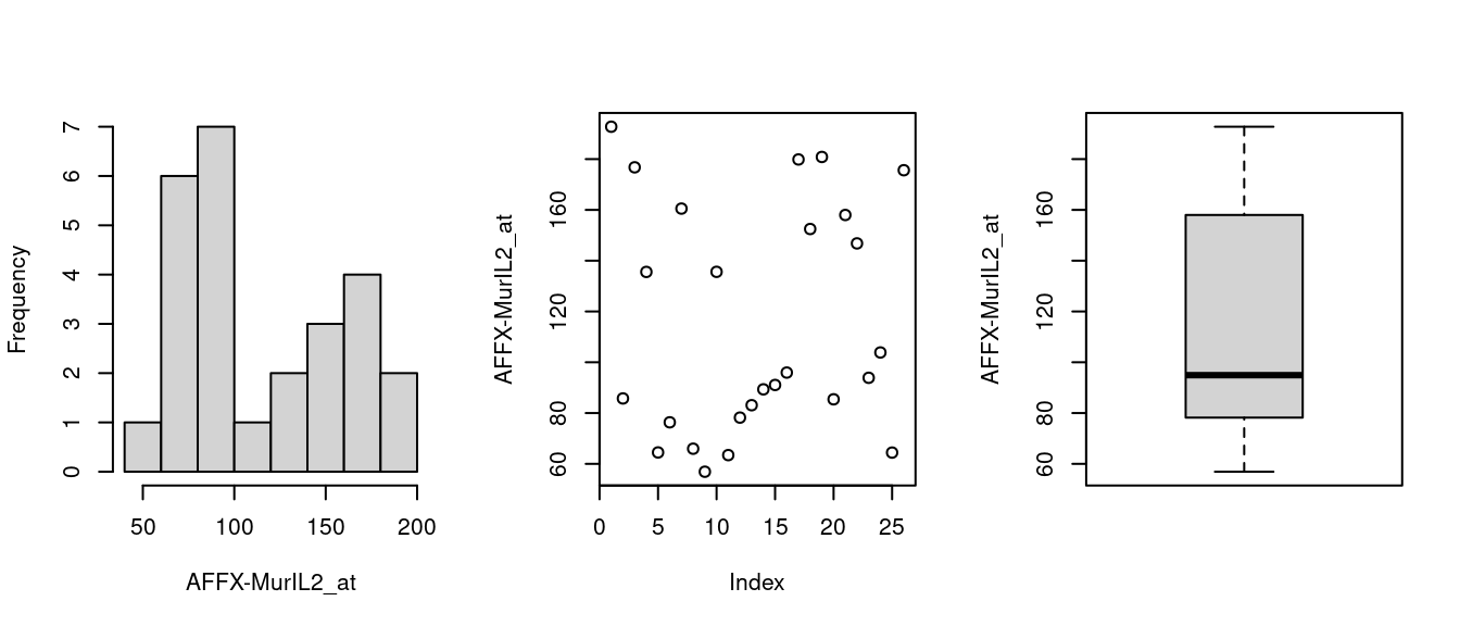
Figure 1.1: Histogram, scatter & boxplots

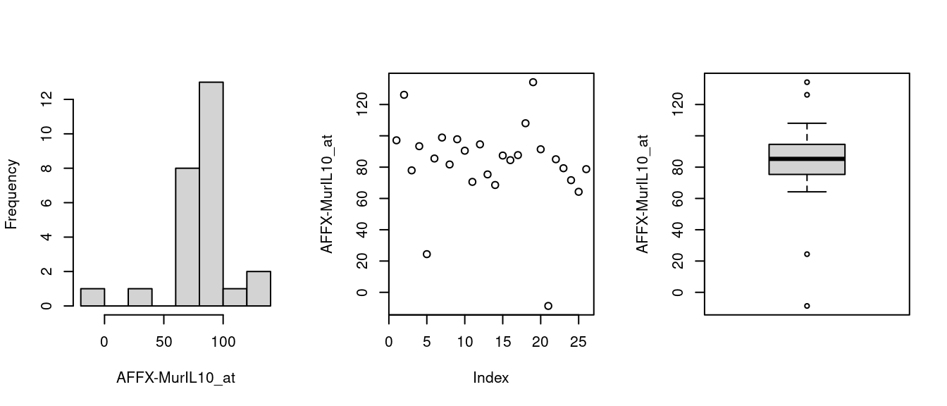
Figure 1.2: Histogram, scatter & boxplots

where the expression set is indexed using feature name(s).

1.3 Outlier detections

This illustrates one mechanism,

list_outliers <- function(es, method="upperquartile")
                 arrayQualityMetrics::outliers(exprs(es),method=method)
for (method in c("KS","sum","upperquartile"))
{
  ZWK_outliers <- list_outliers(protein_ZWK,method=method)
  print(ZWK_outliers@statistic[ZWK_outliers@which])
}

1.4 Clustering

We employ model-based clustering absed on principal compoents to see potential groupings in the data,

  pca <- prcomp(na.omit(t(Biobase::exprs(exampleSet))), rank=10, scale=TRUE)
  pc1pc2pc3 <- with(pca,x)[,1:3]
  mc <- mclust::Mclust(pc1pc2pc3,G=3)
  with(mc, {
      cols <- c("blue","red", "purple")
      s3d <- scatterplot3d::scatterplot3d(with(pca,x[,c(2,1,3)]),
                                          color=cols[classification],
                                          pch=16,
                                          type="h",
                                          main="Plot of the PC1, PC2 and PC3")
      s3d.coords <- s3d$xyz.convert(with(pca,x[,c(2,1,3)]))
      text(s3d.coords$x, 
           s3d.coords$y,   
           cex = 1.2,
           col = cols[classification],
           labels = row.names(pc1pc2pc3),
           pos = 4)
      legend("right", legend=levels(as.factor(classification)), col=cols[classification], pch=16)
      rgl::open3d(width = 500, height = 500)
      rgl::plot3d(with(pca,x[,c(2,1,3)]),cex=1.2,col=cols[classification],size=5)
      rgl::text3d(with(pca,x[,c(2,1,3)]),cex=1.2,col=cols[classification],texts=row.names(pc1pc2pc3))
      htmlwidgets::saveWidget(rgl::rglwidget(), file = "mcpca3d.html")
  })

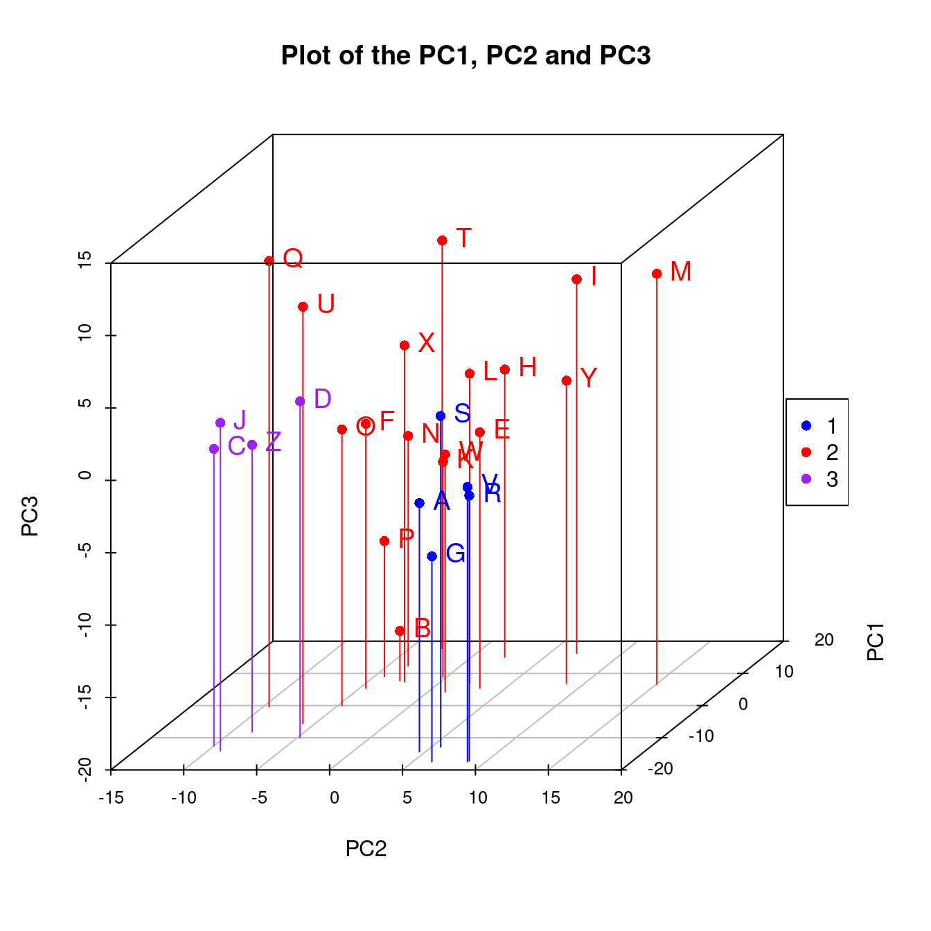
Figure 1.3: Three-group Clustering

#> Warning in par3d(userMatrix = structure(c(1, 0, 0, 0, 0, 0.342020143325668, :
#> parameter "width" cannot be set
#> Warning in par3d(userMatrix = structure(c(1, 0, 0, 0, 0, 0.342020143325668, :
#> parameter "height" cannot be set

An interactive version is also available,

1.5 Data transformation

Suppose we wish use log2 for those greater than zero but set those negative values to be missing.

log2.na <- function(x) log2(ifelse(x>0, x, NA))
Biobase::exprs(exampleSet) <- log2.na(Biobase::exprs(exampleSet))

1.6 Limit of detection (LOD)

We generate a lod.max ~ U[0,1] variable to experiment

Biobase::fData(exampleSet)
#> data frame with 0 columns and 500 rows
Biobase::fData(exampleSet)$lod.max <- apply(Biobase::exprs(exampleSet),1,quantile,runif(nrow(exampleSet)))
lod <- pQTLtools::get.prop.below.LLOD(exampleSet)
x <- dplyr::arrange(Biobase::fData(lod),desc(pc.belowLOD.new))
knitr::kable(head(lod))

	AFFX.MurIL2_at	AFFX.MurIL10_at	AFFX.MurIL4_at	AFFX.MurFAS_at	AFFX.BioB.5_at	AFFX.BioB.M_at	gender	type	score
A	192.7420	97.13700	45.81920	22.54450	96.7875	89.0730	Female	Control	0.75
B	85.7533	126.19600	8.83135	3.60093	30.4380	25.8461	Male	Case	0.40
C	176.7570	77.92160	33.06320	14.68830	46.1271	57.2033	Male	Control	0.73
D	135.5750	93.37130	28.70720	12.33970	70.9319	69.9766	Male	Case	0.42
E	64.4939	24.39860	5.94492	36.86630	56.1744	49.5822	Female	Case	0.93
F	76.3569	85.50880	28.29250	11.25680	42.6756	26.1262	Male	Control	0.22
G	160.5050	98.90860	30.96940	23.00340	86.5156	75.0083	Male	Case	0.96
H	65.9631	81.69320	14.79230	16.21340	30.7927	42.3352	Male	Case	0.79
I	56.9039	97.80150	14.23990	12.03750	19.7183	41.1207	Female	Case	0.37
J	135.6080	90.48380	34.48740	4.54978	46.3520	91.5307	Male	Control	0.63
K	63.4432	70.57330	20.35210	8.51782	39.1326	39.9136	Male	Case	0.26
L	78.2126	94.54180	14.15540	27.28520	41.7698	49.8397	Female	Control	0.36
M	83.0943	75.34550	20.62510	10.16160	80.2197	63.4794	Male	Case	0.41
N	89.3372	68.58270	15.92310	20.24880	36.4903	24.7007	Male	Case	0.80
O	91.0615	87.40500	20.15790	15.78490	36.4021	47.4641	Female	Case	0.10
P	95.9377	84.45810	27.81390	14.32760	35.3054	47.3578	Female	Control	0.41
Q	179.8450	87.68060	32.79110	15.94880	58.6239	58.1331	Female	Case	0.16
R	152.4670	108.03200	33.52920	14.67530	114.0620	104.1220	Male	Control	0.72
S	180.8340	134.26300	19.81720	-7.91911	93.4402	115.8310	Male	Case	0.17
T	85.4146	91.40310	20.41900	12.88750	22.5168	58.1224	Female	Case	0.74
U	157.9890	-8.68811	26.87200	11.91860	48.6462	73.4221	Male	Control	0.35
V	146.8000	85.02120	31.14880	12.83240	90.2215	64.6066	Female	Control	0.77
W	93.8829	79.29980	22.34200	11.13900	42.0053	40.3068	Male	Control	0.27
X	103.8550	71.65520	19.01350	7.55564	57.5738	41.8209	Male	Control	0.98
Y	64.4340	64.23690	12.16860	19.98490	44.8216	46.1087	Female	Case	0.94
Z	175.6150	78.70680	17.37800	8.96849	61.7044	49.4122	Female	Case	0.32

plot(x[,2], main="Random quantile cutoff", ylab="<lod%")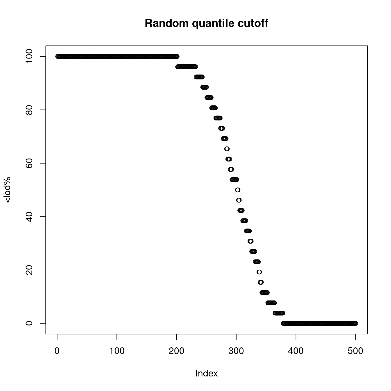

Figure 1.4: LOD based on a random cutoff

The quantity has been shown to have a big impact on protein abundance and therefore pQTL detection as is shown with a real example.

rm(list=ls())
dir <- "~/rds/post_qc_data/interval/phenotype/olink_proteomics/post-qc/"
eset <- readRDS(paste0(dir,"eset.inf1.flag.out.outlier.in.rds"))
x <- pQTLtools::get.prop.below.LLOD(eset)
annot <- Biobase::fData(x)
annot$MissDataProp <- as.numeric(gsub("\\%$", "", annot$MissDataProp))
plot(annot$MissDataProp, annot$pc.belowLOD.new, xlab="% <LLOD in Original",
     ylab="% <LLOD in post QC dataset", pch=19)
INF <- Sys.getenv("INF")
np <- read.table(paste(INF, "work", "INF1.merge.nosig", sep="/"), header=FALSE,
                 col.names = c("prot", "uniprot"))
kable(np, caption="Proteins with no pQTL")
annot$pQTL <- rep(NA, nrow(annot))
no.pQTL.ind <- which(annot$uniprot.id %in% np$uniprot)
annot$pQTL[no.pQTL.ind] <- "red"
annot$pQTL[-no.pQTL.ind] <- "blue"
annot <- annot[order(annot$pc.belowLOD.new, decreasing = TRUE),]
annot <- annot[-grep("^BDNF$", annot$ID),]
saveRDS(annot,file=file.path("~","pQTLtools","tests","annot.RDS"))

annot <- readRDS(file.path(find.package("pQTLtools"),"tests","annot.RDS")) %>%
         dplyr::left_join(pQTLdata::inf1[c("prot","target.short","alt_name")],by=c("ID"="prot")) %>%
         dplyr::mutate(prot=if_else(is.na(alt_name),target.short,alt_name),order=1:n()) %>%
         dplyr::arrange(desc(order))
xtick <- seq(1, nrow(annot))
attach(annot)
par(mar=c(10,5,1,1))
plot(100-pc.belowLOD.new,cex=2,pch=19,col=pQTL,xaxt="n",xlab="",ylab="",cex.axis=0.8)
text(66,16,"IL-17C",offset=0,pos=2,cex=1.5,font=2,srt=0)
arrows(67,16,71,16,lwd=2)
axis(1, at=xtick, labels=prot, lwd.tick=0.5, lwd=0, las=2, hadj=1, cex.axis=0.8)
mtext("% samples above LLOD",side=2,line=2.5,cex=1.2)
mtext("Ordered protein",side=1,line=6.5,cex=1.2,font=1)
legend(x=1,y=25,c("without pQTL","with pQTL"),box.lwd=0,cex=2,col=c("red","blue"),pch=19)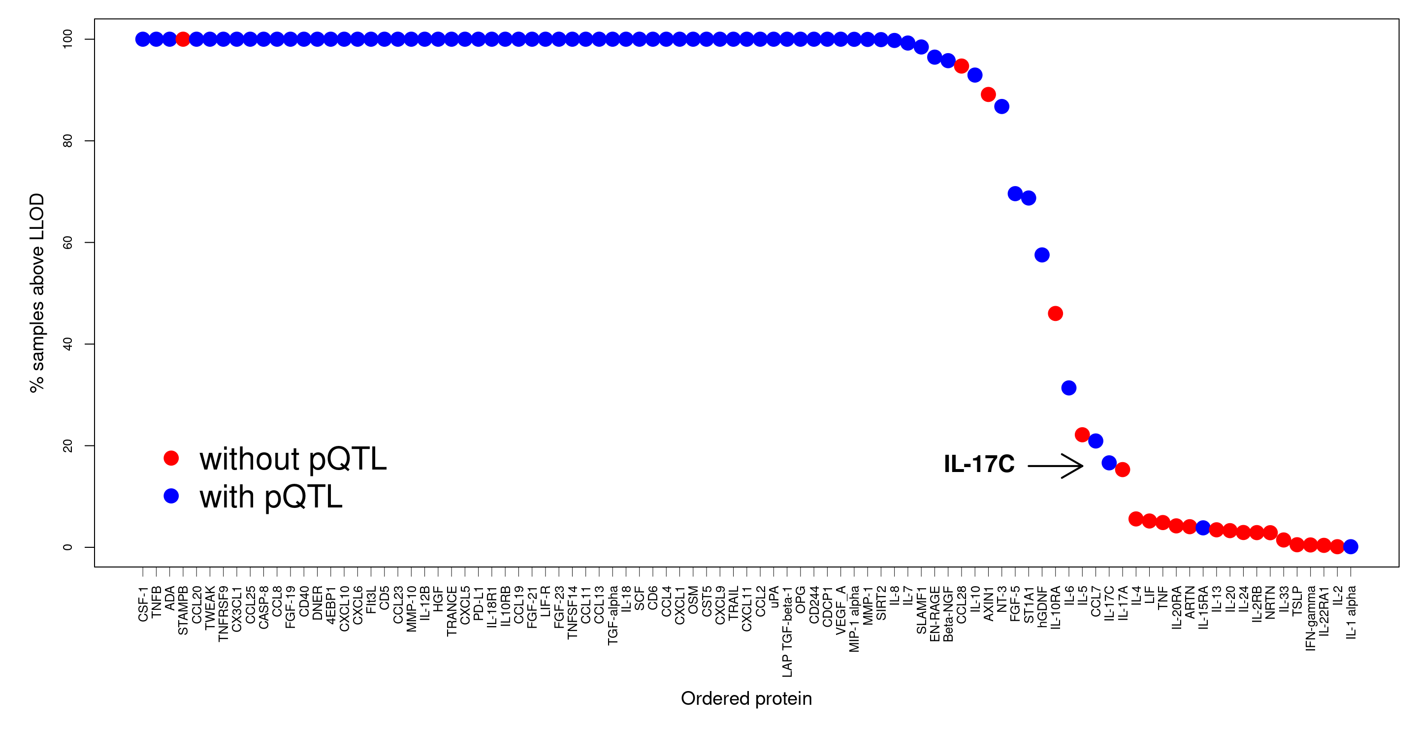

Figure 1.5: LOD in SCALLOP-INF/INTERVAL

detach(annot)
options(width=120)
knitr::kable(annot,caption="Summary statistics",row.names=FALSE)

Table 1.1: Summary statistics
ID	dichot	olink.id	uniprot.id	lod.max	MissDataProp	pc.belowLOD.new	pQTL	target.short	alt_name	prot	order
CSF.1	FALSE	196_CSF-1	P09603	1.02	0.02	0.0000000	blue	CSF-1	NA	CSF-1	91
TNFB	FALSE	195_TNFB	P01374	1.10	0.04	0.0000000	blue	TNFB	NA	TNFB	90
ADA	FALSE	194_ADA	P00813	1.80	0.04	0.0000000	blue	ADA	NA	ADA	89
STAMPB	FALSE	192_STAMPB	O95630	1.40	0.06	0.0000000	red	STAMPB	NA	STAMPB	88
CCL20	FALSE	190_CCL20	P78556	1.42	0.02	0.0000000	blue	CCL20	NA	CCL20	87
TWEAK	FALSE	189_TWEAK	O43508	1.78	0.02	0.0000000	blue	TWEAK	NA	TWEAK	86
TNFRSF9	FALSE	187_TNFRSF9	Q07011	1.86	0.02	0.0000000	blue	TNFRSF9	NA	TNFRSF9	85
CX3CL1	FALSE	186_CX3CL1	P78423	1.76	0.02	0.0000000	blue	CX3CL1	NA	CX3CL1	84
CCL25	FALSE	185_CCL25	O15444	1.32	0.02	0.0000000	blue	CCL25	NA	CCL25	83
CASP.8	FALSE	184_CASP-8	Q14790	1.38	0.04	0.0000000	blue	CASP-8	NA	CASP-8	82
MCP.2	FALSE	183_MCP-2	P80075	2.10	0.02	0.0000000	blue	MCP-2	CCL8	CCL8	81
FGF.19	FALSE	179_FGF-19	O95750	1.25	0.02	0.0000000	blue	FGF-19	NA	FGF-19	80
CD40	FALSE	176_CD40	P25942	1.91	0.04	0.0000000	blue	CD40	NA	CD40	79
DNER	FALSE	174_DNER	Q8NFT8	1.63	0.02	0.0000000	blue	DNER	NA	DNER	78
4E.BP1	FALSE	170_4E-BP1	Q13541	1.04	0.10	0.0000000	blue	4EBP1	NA	4EBP1	77
CXCL10	FALSE	169_CXCL10	P02778	2.03	0.02	0.0000000	blue	CXCL10	NA	CXCL10	76
CXCL6	FALSE	168_CXCL6	P80162	1.80	0.02	0.0000000	blue	CXCL6	CXCL6	CXCL6	75
Flt3L	FALSE	167_Flt3L	P49771	2.12	0.02	0.0000000	blue	FIt3L	NA	FIt3L	74
CD5	FALSE	165_CD5	P06127	1.42	0.02	0.0000000	blue	CD5	NA	CD5	73
CCL23	FALSE	164_CCL23	P55773	2.10	0.02	0.0000000	blue	CCL23	NA	CCL23	72
MMP.10	FALSE	161_MMP-10	P09238	1.56	0.02	0.0000000	blue	MMP-10	NA	MMP-10	71
IL.12B	FALSE	157_IL-12B	P29460	0.85	0.02	0.0000000	blue	IL-12B	NA	IL-12B	70
HGF	FALSE	156_HGF	P14210	1.77	0.02	0.0000000	blue	HGF	NA	HGF	69
TRANCE	FALSE	155_TRANCE	O14788	1.51	0.04	0.0000000	blue	TRANCE	NA	TRANCE	68
CXCL5	FALSE	154_CXCL5	P42830	1.92	0.02	0.0000000	blue	CXCL5	NA	CXCL5	67
PD.L1	FALSE	152_PD-L1	Q9NZQ7	2.14	0.04	0.0000000	blue	PD-L1	NA	PD-L1	66
IL.18R1	FALSE	151_IL-18R1	Q13478	1.21	0.02	0.0000000	blue	IL-18R1	NA	IL-18R1	65
IL.10RB	FALSE	149_IL-10RB	Q08334	1.72	0.02	0.0000000	blue	IL10RB	NA	IL10RB	64
CCL19	FALSE	145_CCL19	Q99731	2.13	0.02	0.0000000	blue	CCL19	NA	CCL19	63
FGF.21	FALSE	144_FGF-21	Q9NSA1	1.14	0.02	0.0000000	blue	FGF-21	NA	FGF-21	62
LIF.R	FALSE	143_LIF-R	P42702	2.08	0.04	0.0000000	blue	LIF-R	NA	LIF-R	61
FGF.23	FALSE	139_FGF-23	Q9GZV9	0.66	0.04	0.0000000	blue	FGF-23	NA	FGF-23	60
TNFSF14	FALSE	138_TNFSF14	O43557	1.81	0.02	0.0000000	blue	TNFSF14	NA	TNFSF14	59
CCL11	FALSE	137_CCL11	P51671	2.09	0.02	0.0000000	blue	CCL11	CCL11	CCL11	58
MCP.4	FALSE	136_MCP-4	Q99616	0.56	0.04	0.0000000	blue	MCP-4	CCL13	CCL13	57
TGF.alpha	FALSE	135_TGF-alpha	P01135	0.07	0.02	0.0000000	blue	TGF-alpha	NA	TGF-alpha	56
IL.18	FALSE	133_IL-18	Q14116	2.79	0.02	0.0000000	blue	IL-18	NA	IL-18	55
SCF	FALSE	132_SCF	P21583	2.30	0.02	0.0000000	blue	SCF	NA	SCF	54
CD6	FALSE	131_CD6	Q8WWJ7	1.78	0.04	0.0000000	blue	CD6	NA	CD6	53
CCL4	FALSE	130_CCL4	P13236	2.15	0.02	0.0000000	blue	CCL4	NA	CCL4	52
CXCL1	FALSE	128_CXCL1	P09341	3.45	0.02	0.0000000	blue	CXCL1	NA	CXCL1	51
OSM	FALSE	126_OSM	P13725	1.32	0.06	0.0000000	blue	OSM	NA	OSM	50
CST5	FALSE	123_CST5	P28325	4.34	0.04	0.0000000	blue	CST5	NA	CST5	49
CXCL9	FALSE	122_CXCL9	Q07325	1.04	0.02	0.0000000	blue	CXCL9	NA	CXCL9	48
TRAIL	FALSE	120_TRAIL	P50591	1.22	0.02	0.0000000	blue	TRAIL	NA	TRAIL	47
CXCL11	FALSE	117_CXCL11	O14625	1.40	0.02	0.0000000	blue	CXCL11	NA	CXCL11	46
MCP.1	FALSE	115_MCP-1	P13500	1.90	0.02	0.0000000	blue	MCP-1	CCL2	CCL2	45
uPA	FALSE	112_uPA	P00749	1.75	0.02	0.0000000	blue	uPA	NA	uPA	44
LAP.TGF.beta.1	FALSE	111_LAP TGF-beta-1	P01137	0.86	0.02	0.0000000	blue	LAP TGF-beta-1	NA	LAP TGF-beta-1	43
OPG	FALSE	110_OPG	O00300	1.81	0.02	0.0000000	blue	OPG	NA	OPG	42
CD244	FALSE	108_CD244	Q9BZW8	1.09	0.02	0.0000000	blue	CD244	NA	CD244	41
CDCP1	FALSE	107_CDCP1	Q9H5V8	0.21	0.04	0.0000000	blue	CDCP1	NA	CDCP1	40
VEGF.A	FALSE	102_VEGF-A	P15692	3.15	0.02	0.0000000	blue	VEGF_A	NA	VEGF_A	39
MIP.1.alpha	FALSE	166_MIP-1 alpha	P10147	1.92	0.06	0.0203998	blue	MIP-1 alpha	NA	MIP-1 alpha	38
MMP.1	FALSE	142_MMP-1	P03956	1.89	0.06	0.0407997	blue	MMP-1	NA	MMP-1	37
SIRT2	FALSE	172_SIRT2	Q8IXJ6	1.52	1.00	0.0815993	blue	SIRT2	NA	SIRT2	36
IL.8	FALSE	101_IL-8	P10145	3.17	0.25	0.2447980	blue	IL-8	NA	IL-8	35
IL.7	FALSE	109_IL-7	P13232	1.39	1.43	0.7547940	blue	IL-7	NA	IL-7	34
SLAMF1	FALSE	134_SLAMF1	Q13291	1.55	2.13	1.5299878	blue	SLAMF1	NA	SLAMF1	33
EN.RAGE	FALSE	175_EN-RAGE	P80511	1.57	3.28	3.5291718	blue	EN-RAGE	NA	EN-RAGE	32
Beta.NGF	FALSE	153_Beta-NGF	P01138	1.23	3.96	4.2227662	blue	Beta-NGF	NA	Beta-NGF	31
CCL28	FALSE	173_CCL28	Q9NRJ3	0.92	5.49	5.2835577	red	CCL28	NA	CCL28	30
IL.10	FALSE	162_IL-10	P22301	1.50	7.71	7.0583435	blue	IL-10	NA	IL-10	29
AXIN1	FALSE	118_AXIN1	O15169	1.30	13.04	10.8731130	red	AXIN1	NA	AXIN1	28
NT.3	FALSE	188_NT-3	P20783	0.85	12.77	13.2394941	blue	NT-3	NA	NT-3	27
FGF.5	FALSE	141_FGF-5	Q8NF90	1.00	31.71	30.3957568	blue	FGF-5	NA	FGF-5	26
ST1A1	FALSE	191_ST1A1	P50225	1.34	32.68	31.2525500	blue	ST1A1	NA	ST1A1	25
GDNF	FALSE	106_GDNF	P39905	1.13	43.26	42.4520604	blue	hGDNF	NA	hGDNF	24
IL.10RA	FALSE	140_IL-10RA	Q13651	1.14	53.30	53.9779682	red	IL-10RA	NA	IL-10RA	23
IL.6	FALSE	113_IL-6	P05231	1.97	69.06	68.6250510	blue	IL-6	NA	IL-6	22
IL.5	FALSE	193_IL-5	P05113	1.55	78.21	77.8457772	red	IL-5	NA	IL-5	21
MCP.3	FALSE	105_MCP-3	P80098	1.31	79.30	79.0697674	blue	MCP-3	CCL7	CCL7	20
IL.17C	FALSE	114_IL-17C	Q9P0M4	1.28	83.07	83.3741330	blue	IL-17C	NA	IL-17C	19
IL.17A	FALSE	116_IL-17A	Q16552	0.97	84.73	84.7001224	red	IL-17A	NA	IL-17A	18
IL.4	FALSE	180_IL-4	P05112	1.11	93.91	94.4104447	red	IL-4	NA	IL-4	17
LIF	FALSE	181_LIF	P15018	1.45	94.90	94.8184415	red	LIF	NA	LIF	16
TNF	FALSE	163_TNF	P01375	1.19	95.22	95.1244390	red	TNF	NA	TNF	15
IL.20RA	FALSE	121_IL-20RA	Q9UHF4	0.79	95.16	95.7772338	red	IL-20RA	NA	IL-20RA	14
ARTN	FALSE	160_ARTN	Q5T4W7	0.73	95.84	95.9404325	red	ARTN	NA	ARTN	13
IL.15RA	FALSE	148_IL-15RA	Q13261	1.18	96.10	96.1648307	blue	IL-15RA	NA	IL-15RA	12
IL.13	FALSE	159_IL-13	P35225	1.71	96.51	96.5524276	red	IL-13	NA	IL-13	11
IL.20	FALSE	171_IL-20	Q9NYY1	1.30	96.72	96.7156263	red	IL-20	NA	IL-20	10
IL.24	FALSE	158_IL-24	Q13007	1.95	97.13	97.0828233	red	IL-24	NA	IL-24	9
IL.2RB	FALSE	124_IL-2RB	P14784	1.47	97.11	97.1032232	red	IL-2RB	NA	IL-2RB	8
NRTN	FALSE	182_NRTN	Q99748	1.39	97.11	97.1236230	red	NRTN	NA	NRTN	7
IL.33	FALSE	177_IL-33	O95760	1.17	98.54	98.5516116	red	IL-33	NA	IL-33	6
TSLP	FALSE	129_TSLP	Q969D9	1.80	99.49	99.4900041	red	TSLP	NA	TSLP	5
IFN.gamma	FALSE	178_IFN-gamma	P01579	1.40	99.53	99.5308038	red	IFN-gamma	NA	IFN-gamma	4
IL.22.RA1	FALSE	150_IL-22 RA1	Q8N6P7	1.79	99.61	99.6124031	red	IL-22RA1	NA	IL-22RA1	3
IL.2	FALSE	127_IL-2	P60568	0.93	99.86	99.8776010	red	IL-2	NA	IL-2	2
IL.1.alpha	FALSE	125_IL-1 alpha	P01583	4.76	99.88	99.8776010	blue	IL-1 alpha	NA	IL-1 alpha	1

1.7 maEndtoEnd

Web: https://bioconductor.org/packages/release/workflows/html/maEndToEnd.html.

Examples can be found on PCA, heatmap, normalisation, linear models, and enrichment analysis from this Bioconductor package.

2 SummarizedExperiment

This is a more modern construct. Based on the documentation example, ranged summarized experiment (rse) and imputation are shown below.

set.seed(123)
nrows <- 20
ncols <- 4
counts <- matrix(runif(nrows * ncols, 1, 1e4), nrows)
missing_indices <- sample(length(counts), size = 5, replace = FALSE)
counts[missing_indices] <- NA
rowRanges <- GenomicRanges::GRanges(rep(c("chr1", "chr2"), c(1, 3) * nrows / 4),
                            IRanges::IRanges(floor(runif(nrows, 1e5, 1e6)), width=ncols),
                            strand=sample(c("+", "-"), nrows, TRUE),
                            feature_id=sprintf("ID%03d", 1:nrows))
colData <- S4Vectors::DataFrame(Treatment=rep(c("ChIP", "Input"), ncols/2),
                                row.names=LETTERS[1:ncols])
rse <- SummarizedExperiment(assays=S4Vectors::SimpleList(counts=counts),
                            rowRanges=rowRanges, colData=colData)
assay(rse)
#>               A         B         C           D
#>  [1,] 2876.4876 8895.5036 1428.8574 6651.486831
#>  [2,] 7883.2630 6928.3413 4146.0488  949.311769
#>  [3,] 4090.3602 6405.4276 4137.8295 3840.312408
#>  [4,] 8830.2910 9942.7035 3689.0857 2744.562062
#>  [5,] 9404.7324 6557.4023 1525.2950 8146.585749
#>  [6,]        NA 7085.5962 1388.9218 4485.714898
#>  [7,] 5281.5268 5441.1162 2331.1080 8100.833466
#>  [8,] 8924.2980 5941.8261 4660.1585 8124.082706
#>  [9,] 5514.7987 2892.3082 2660.4604 7943.628869
#> [10,] 4566.6907 1471.9894        NA 4398.877044
#> [11,] 9568.3766        NA  459.2658 7544.997111
#> [12,] 4533.8882 9023.0882 4422.5585          NA
#> [13,] 6776.0288 6907.3621 7989.4495 7102.113831
#> [14,] 5726.7614 7954.8787 1219.8707    7.247108
#> [15,] 1030.1439  247.1122 5609.9189 4753.690424
#> [16,] 8998.3499 4778.4819 2066.1074 2201.968733
#> [17,] 2461.6313 7584.8369 1276.1890 3798.785561
#> [18,]  421.5533 2164.8630 7533.3253 6128.097262
#> [19,] 3279.8793        NA 8950.5585 3518.627295
#> [20,] 9545.0820 2317.0262 3745.2533 1112.243108
imputed <- MsCoreUtils::impute_knn(as.matrix(SummarizedExperiment::assay(rse)),2)
imputed_counts <- MsCoreUtils::impute_RF(as.matrix(assay(rse)),2)
imputed-imputed_counts
#>              A         B        C        D
#>  [1,]    0.000    0.0000    0.000    0.000
#>  [2,]    0.000    0.0000    0.000    0.000
#>  [3,]    0.000    0.0000    0.000    0.000
#>  [4,]    0.000    0.0000    0.000    0.000
#>  [5,]    0.000    0.0000    0.000    0.000
#>  [6,] 2559.339    0.0000    0.000    0.000
#>  [7,]    0.000    0.0000    0.000    0.000
#>  [8,]    0.000    0.0000    0.000    0.000
#>  [9,]    0.000    0.0000    0.000    0.000
#> [10,]    0.000    0.0000 1791.909    0.000
#> [11,]    0.000 -709.2786    0.000    0.000
#> [12,]    0.000    0.0000    0.000 2467.614
#> [13,]    0.000    0.0000    0.000    0.000
#> [14,]    0.000    0.0000    0.000    0.000
#> [15,]    0.000    0.0000    0.000    0.000
#> [16,]    0.000    0.0000    0.000    0.000
#> [17,]    0.000    0.0000    0.000    0.000
#> [18,]    0.000    0.0000    0.000    0.000
#> [19,]    0.000 1298.3456    0.000    0.000
#> [20,]    0.000    0.0000    0.000    0.000
SummarizedExperiment::assays(rse) <- S4Vectors::SimpleList(counts=imputed_counts)
SummarizedExperiment::assay(rse)
#>               A         B         C           D
#>  [1,] 2876.4876 8895.5036 1428.8574 6651.486831
#>  [2,] 7883.2630 6928.3413 4146.0488  949.311769
#>  [3,] 4090.3602 6405.4276 4137.8295 3840.312408
#>  [4,] 8830.2910 9942.7035 3689.0857 2744.562062
#>  [5,] 9404.7324 6557.4023 1525.2950 8146.585749
#>  [6,] 4439.2947 7085.5962 1388.9218 4485.714898
#>  [7,] 5281.5268 5441.1162 2331.1080 8100.833466
#>  [8,] 8924.2980 5941.8261 4660.1585 8124.082706
#>  [9,] 5514.7987 2892.3082 2660.4604 7943.628869
#> [10,] 4566.6907 1471.9894 4812.3872 4398.877044
#> [11,] 9568.3766 5545.7565  459.2658 7544.997111
#> [12,] 4533.8882 9023.0882 4422.5585 4611.837102
#> [13,] 6776.0288 6907.3621 7989.4495 7102.113831
#> [14,] 5726.7614 7954.8787 1219.8707    7.247108
#> [15,] 1030.1439  247.1122 5609.9189 4753.690424
#> [16,] 8998.3499 4778.4819 2066.1074 2201.968733
#> [17,] 2461.6313 7584.8369 1276.1890 3798.785561
#> [18,]  421.5533 2164.8630 7533.3253 6128.097262
#> [19,] 3279.8793 4566.2289 8950.5585 3518.627295
#> [20,] 9545.0820 2317.0262 3745.2533 1112.243108
SummarizedExperiment::assays(rse) <- S4Vectors::endoapply(SummarizedExperiment::assays(rse), asinh)
SummarizedExperiment::assay(rse)
#>              A        B        C        D
#>  [1,] 8.657472 9.786448 7.957778 9.495743
#>  [2,] 9.665644 9.536523 9.023058 7.548885
#>  [3,] 9.009536 9.458048 9.021074 8.946456
#>  [4,] 9.779090 9.897741 8.906281 8.610524
#>  [5,] 9.842115 9.481497 8.023090 9.698501
#>  [6,] 9.091398 9.558966 7.929430 9.101800
#>  [7,] 9.265118 9.294887 8.447246 9.692869
#>  [8,] 9.789680 9.382919 9.139952 9.695735
#>  [9,] 9.308338 8.662957 8.579402 9.673273
#> [10,] 9.119691 7.987517 9.172096 9.082252
#> [11,] 9.859366 9.313936 6.822778 9.621787
#> [12,] 9.112482 9.800689 9.087621 9.129529
#> [13,] 9.514294 9.533490 9.679024 9.561295
#> [14,] 9.346053 9.674688 7.799647 2.678476
#> [15,] 7.630601 6.202994 9.325439 9.159824
#> [16,] 9.797944 9.165025 8.326569 8.390254
#> [17,] 8.501727 9.627054 7.844781 8.935584
#> [18,] 6.737095 8.373260 9.620239 9.413787
#> [19,] 8.788709 9.119590 9.792618 8.858973
#> [20,] 9.856929 8.441187 8.921392 7.707281

SummarizedExperiment::rowRanges(rse)
#> GRanges object with 20 ranges and 1 metadata column:
#>        seqnames        ranges strand |  feature_id
#>           <Rle>     <IRanges>  <Rle> | <character>
#>    [1]     chr1 409164-409167      - |       ID001
#>    [2]     chr1 691082-691085      + |       ID002
#>    [3]     chr1 388335-388338      + |       ID003
#>    [4]     chr1 268922-268925      - |       ID004
#>    [5]     chr1 804064-804067      - |       ID005
#>    ...      ...           ...    ... .         ...
#>   [16]     chr2 647861-647864      + |       ID016
#>   [17]     chr2 469620-469623      + |       ID017
#>   [18]     chr2 232385-232388      + |       ID018
#>   [19]     chr2 941769-941772      - |       ID019
#>   [20]     chr2 371106-371109      + |       ID020
#>   -------
#>   seqinfo: 2 sequences from an unspecified genome; no seqlengths
SummarizedExperiment::rowData(rse)
#> DataFrame with 20 rows and 1 column
#>      feature_id
#>     <character>
#> 1         ID001
#> 2         ID002
#> 3         ID003
#> 4         ID004
#> 5         ID005
#> ...         ...
#> 16        ID016
#> 17        ID017
#> 18        ID018
#> 19        ID019
#> 20        ID020
SummarizedExperiment::colData(rse)
#> DataFrame with 4 rows and 1 column
#>     Treatment
#>   <character>
#> A        ChIP
#> B       Input
#> C        ChIP
#> D       Input

rse[, rse$Treatment == "ChIP"]
#> class: RangedSummarizedExperiment 
#> dim: 20 2 
#> metadata(0):
#> assays(1): counts
#> rownames: NULL
#> rowData names(1): feature_id
#> colnames(2): A C
#> colData names(1): Treatment

# the same ranges but different samples:
rse1 <- rse
rse2 <- rse1[, 1:3]
colnames(rse2) <- letters[1:ncol(rse2)]
cmb1 <- cbind(rse1, rse2)
dim(cmb1)
#> [1] 20  7
dimnames(cmb1)
#> [[1]]
#> NULL
#> 
#> [[2]]
#> [1] "A" "B" "C" "D" "a" "b" "c"

# the same samples but different ranges:
rse1 <- rse
rse2 <- rse1[1:nrows, ]
rownames(rse2) <- letters[1:nrow(rse2)]
cmb2 <- rbind(rse1, rse2)
dim(cmb2)
#> [1] 40  4
dimnames(cmb2)
#> [[1]]
#>  [1] ""  ""  ""  ""  ""  ""  ""  ""  ""  ""  ""  ""  ""  ""  ""  ""  ""  ""  ""  ""  "a" "b" "c" "d" "e" "f" "g" "h" "i"
#> [30] "j" "k" "l" "m" "n" "o" "p" "q" "r" "s" "t"
#> 
#> [[2]]
#> [1] "A" "B" "C" "D"

se0 <- as(rse, "SummarizedExperiment")
se0
#> class: SummarizedExperiment 
#> dim: 20 4 
#> metadata(0):
#> assays(1): counts
#> rownames: NULL
#> rowData names(1): feature_id
#> colnames(4): A B C D
#> colData names(1): Treatment
as(se0, "RangedSummarizedExperiment")
#> class: RangedSummarizedExperiment 
#> dim: 20 4 
#> metadata(0):
#> assays(1): counts
#> rownames: NULL
#> rowData names(1): feature_id
#> colnames(4): A B C D
#> colData names(1): Treatment

# rowRanges(a SummarizedExperiment object) --> RangedSummarizedExperiment object:
se <- se0
rowRanges(se) <- rowRanges
se
#> class: RangedSummarizedExperiment 
#> dim: 20 4 
#> metadata(0):
#> assays(1): counts
#> rownames: NULL
#> rowData names(1): feature_id
#> colnames(4): A B C D
#> colData names(1): Treatment

stopifnot(identical(SummarizedExperiment::assays(se0), SummarizedExperiment::assays(rse)))
stopifnot(identical(dim(se0), dim(rse)))
stopifnot(identical(dimnames(se0), dimnames(rse)))
stopifnot(identical(SummarizedExperiment::rowData(se0), SummarizedExperiment::rowData(rse)))
stopifnot(identical(SummarizedExperiment::colData(se0), SummarizedExperiment::colData(rse)))